Abstract
This paper presents the development of physics-informed machine learning models for subsurface flows, specifically for determining pressure variation in the subsurface without the use of numerical modeling schemes. The numerical elliptic operator is replaced with a neural network operator and includes comparisons of several different machine learning models, along with linear regression, support vector regression, lasso, random forest regression, decision tree regression, light weight gradient boosting, eXtreme gradient boosting, convolution neural network, artificial neural network, and perceptron. The mean of absolute error of all models is compared, and error residual plots are used as a measure of error to determine the best-performing method.
Highlights
- Predicting Flow in Porous Media
- Data Driven Approach
- Comparison of Several Machine Learning models
- Rigorous analysis
1. Introduction
Over the years, significant progress has been made in understanding multiscale physics through the numerical solution of partial differential equations. However, traditional numerical methods face challenges when dealing with real-world physics problems that have missing or noisy boundary conditions. In contrast, machine learning can explore large design spaces, identify correlations in multi-dimensional data, and manage ill-posed problems.
Deep learning tools [5] are particularly effective at extracting useful information from enormous amounts of data and linking important features with approximate models. They are especially useful for multi-dimensional subsurface flow problems because of their inverse nature. Nevertheless, current machine learning approaches often lack the ability to extract interpretable information and knowledge from the data, leading to poor generalization and physically inconsistent predictions.
To overcome these issues, physics-informed machine learning techniques [1-3] can incorporate physical constraints and domain knowledge into machine learning models. By “teaching” ML models about the governing physical rules, this approach can provide informative priors, such as strong theoretical constraints and inductive biases, that improve the performance of learning algorithms [4]. This process requires physics-based learning, which refers to the use of prior knowledge derived from observational, empirical, physical, or mathematical understanding of the world to improve machine learning algorithms' performance.
Machine learning methods can be categorized into supervised learning, unsupervised learning, and reinforcement learning. Supervised learning involves training a model using labeled input and output data and can be further divided into regression and classification. Examples of regression models include linear regression [6], Lasso [7], support vector regression [8], and random forest regression [9], while examples of classification models include logistic regression [10], naive Bayes classifier, and KNN classifier [11]. Unsupervised learning is used for unlabeled output data, with examples including principal component analysis [12] and singular value decomposition [13]. Reinforcement learning, on the other hand, learns from the environment based on reward and penalty.
In this paper we aim to apply Machine learning models to solve Single-phase Darcy’s flow equation. The Darcy flow equation is given as:
where is permeability or conductivity of the porous medium, – Darcy’s flow velocity, – pressure, – fluid density, – dynamic viscosity of the fluid, – gravitational constant, – spatial direction. The given equation can be solved by assuming constant porosity of the porous media domain and incompressibility, which reduces the equation into an elliptic pressure equation. The elliptic pressure equation’s solution can be approximated via machine learning models. The equation’s solution is relevant for understanding flow in subsurface hydrogeology, hydrocarbon reservoirs, and geothermal systems. In recent times researchers have tried to use machine learning models for modelling porous media flow, a comparative analysis of recent research work is presented in Table 1.
Table 1Comparison of work done in this field
Title | Author | Remark |
Physics-Informed Deep Neural Networks for Learning Parameters and Constitutive Relationships in Subsurface Flow Problems ([1]) | A. M. Tartakovsky, C. Ortiz Marrero, Paris Perdikaris, G. D. Tartakovsky, and D. Barajas-Solano | The authors propose a physics-informed machine learning method for estimating hydraulic conductivity in both saturated and unsaturated flows governed by Darcy’s law. By adding physics constraints to the training of deep neural networks, the accuracy of DNN parameter estimation could increase by up to 50 %. The proposed method uses conservation laws and data to train DNNs representing the state variables, space-dependent coefficients, and constitutive relationships for two specific scenarios: saturated flow in heterogeneous porous media with unknown conductivity and unsaturated flow in homogeneous porous media with an unknown relationship between capillary pressure and unsaturated conductivity. |
Physics-constrained deep learning for data assimilation of subsurface transport ([2]) | Haiyi Wu∗, Rui Qiao∗ | The authors developed a modeling approach that uses sparse measurements of observables to predict full-scale hydraulic conductivity, hydraulic head, and concentration fields in porous media. The structure is described by a system parameter vector and a solution vector, with measurement data that consists of the vectors at the system boundaries and sparse measurements of the vectors inside the system. The goal is to estimate the full-scale system parameter when solution vectors are using the measured data, with an average relative error achieved by the modeling approach of 0.1. |
Computing Challenges in Oil and Gas Field Simulation ([26]) | Jeroen C. Vink | This paper discusses current simulation challenges and emerging computing strategies in the oil and gas industry to accurately model and optimize hydrocarbon production while minimizing environmental impact and maximizing resource recovery. Large-scale computer simulations are critical for mitigating risks associated with developing reservoirs in remote and hostile locations, but current techniques must be improved to meet the demands of today’s reservoirs. This includes simulating larger models with more geological detail, capturing fluid chemistry and thermodynamics in more detail, and reliably estimating uncertainty ranges in simulated results. |
The Neural Upscaling Method for Single-Phase flow in Porous Medium ([27]) | M. Pal, P. Makauskas, P. Saxena, P. Patil | The paper presents the development of a Neural upscaling network for upscaling heterogeneous permeability fields using a feed-forward neural network with hidden layers trained using backpropagation. The Perlin noise function is used to generate a sub-surface permeability distribution, which is applied at each grid level to ensure self-consistency and comparability across resolutions. The algorithm generates a random pattern of values to create smooth, organic-looking surfaces. Mean square error is used to optimize neural network performance. |
Neural solution to elliptic PDE with discontinuous coefficients for flow in porous media ([28]) | M. Pal, P. Makauskas, M. Ragulskis, D. Guerillot | The paper proposes a neural solution method for solving tensor elliptic PDEs with discontinuous coefficients. The method is based on a deep learning multi-layer neural network, which is claimed to be more effective than TPFA [29] or MPFA [29] type schemes. The paper presents a series of 2D test cases, comparing the Neural solution method with numerical solutions using TPFA and MPFA schemes with different degrees of heterogeneity. The accuracy and order of convergence of the method are analyzed, and a physics-informed neural network based on a CNN is proposed to improve accuracy. The method is evaluated on one and two-dimensional cases involving varying degrees of fine-scale permeability heterogeneity, and mean square error is used to optimize the network performance. |
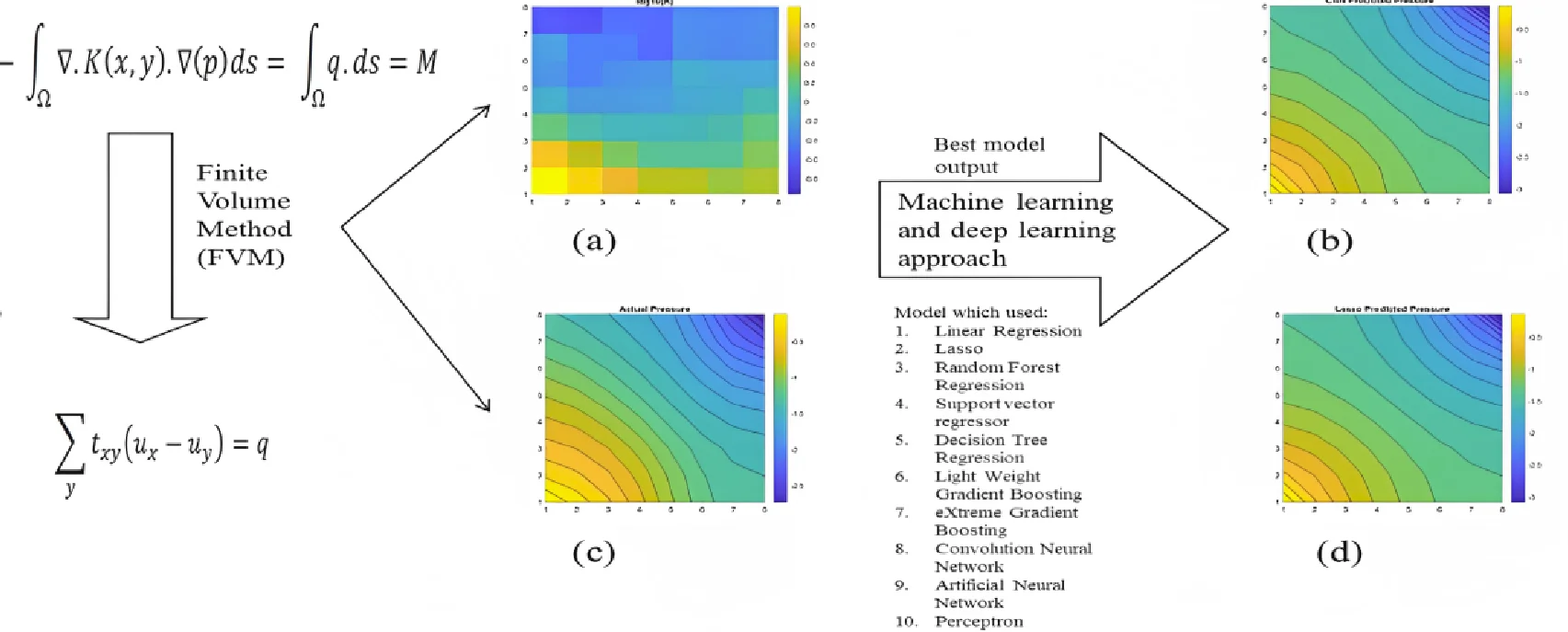
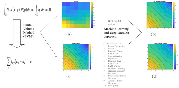
This paper addresses the challenges of numerical simulation for subsurface flow and transport problems in porous media, emphasizing the complexity of domain modeling required for accurate representation of real-world entities and relationships. Traditional numerical simulations involve solving PDEs on a network of networks, which increases computational complexity and necessitates the creation of large matrices. To address this, the paper proposes the use of machine learning as a cost-effective and time-saving alternative for solving these problems. The finite-volume approach generates data for the study, and Fig. 1 shows the permeability distribution and pressure in a 2×8 grid.
The strength of this approach lies in the comparative analysis of several machine learning models for solving single-phase Darcy’s flow equation. The objective is to develop a machine learning model that replicates numerical reservoir simulator outputs for single-phase flow problems, utilizing deep learning tools such as the Perceptron [14], Convolution Neural Network [15-22], and Artificial Neural Network models. The presented models are robust enough to predict pressure variation in the reservoir based on given permeability variations. The proposed approach removes challenges associated with numerical methods such as numerical diffusion, dispersion, and computational cost.
The paper is organized as follows: subsurface flow problem is described in Section 2. Flow equations are described in Section 3. Machine learning methodology used in this paper is described in Section 4. Results are presented in Section 5 and conclusions follow in Section 6.
Fig. 1a) Shows 1-D linear permeability distribution, b) pressure solution on a 2×8 grid
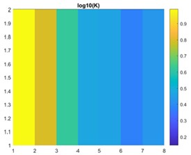
a)
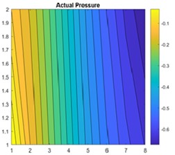
b)
2. Single-phase Darcy flow equation
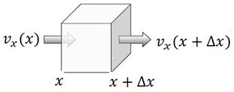
To derive an equation for flow in 1D, we assume that the cross-section area for flow as well as the depth , are functions of the variable in our 1D space. Additionally, we introduce a term for the injection of fluid, which is equal to the mass rate of injection per unit volume of reservoir. Consider a mass balance in a small box shown in Fig. 2. The length of the box is , the left side has area , the right side has area .
Fig. 2Differential elements of volume for a one-dimensional flow
Rate at which fluid mass enters the box at the left face is given by:
Rate at which fluid mass leaves at the right face:
If we define the average value of and between and as and , we get, that the volume of the box is .
Rate at which fluid mass is injected into the box is:
The mass contained in the box is . So, we get the rate of accumulation of mass in the box:
From conservation of mass:
Putting values from Eq. (2-5) in Eq. (6), we yield:
Divided by , assuming area is constant, and taking limit , we will get:
or
Here the source term models sources and sinks, that is, outflow and inflow per volume at designated well locations. For the incompressible single-phase flow assume that the porosity of the rock is constant in time and that the fluid is incompressible, which means density is constant. Then the time dependent derivative vanishes, and we obtain the elliptic equation for the water pressure. Putting value of from Eq. (1) into Eq. (9), we will get:
When solving fluid flow problems, it is common practice to specify boundary conditions to ensure that the system is well-defined, and that the solution is physically meaningful. In this case, a no-flow boundary condition is imposed on the reservoir boundary, which means that the fluid velocity vector must be perpendicular to the boundary, as indicated by the dot product , 0, where n is the normal vector pointing out of the boundary. This condition ensures that no fluid can enter or exit the reservoir through the boundary, and the system is effectively isolated. Other types of boundary conditions, such as constant pressure or velocity, could also be used depending on the specific problem being solved.
2.1. Numerical solution: finite volume approach
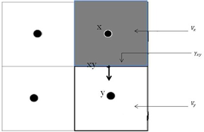
In finite-difference methods, the domain is discretized into a grid of points and the partial derivatives are approximated using difference formulas at each grid point. The solution is then obtained by solving a system of algebraic equations obtained from discretizing the PDE at each grid point. In contrast, the finite-volume method (FVM) divides the computational domain into a finite number of small control volumes, or cells. The fluxes of fluid through the boundaries of each cell are then calculated, and the equation is discretized over the entire domain, see Fig. 3. The resulting set of algebraic equations can be solved using iterative methods to obtain a numerical solution. There are several variations of the FVM, such as the two-point flux method (TPFM) [29] and the multi-point flux method (MPFM) [29], which differ in the way they approximate the fluxes. In the TPFM, the fluxes across each face of a control volume are approximated using a two-point approximation, which assumes that the flux at a face is proportional to the pressure difference between the neighboring control volumes. The TPFM is based on the principle of conservation of flux, which states that the total flux into a control volume must be equal to the total flux out of the control volume.
We derive an equation that models flow of a fluid, say, water (), through a porous medium characterized by a permeability field and corresponding porosity distribution. So, Eq. (10) can be written as:
To derive a set of FV (finite volume) mass-balance equations for Eq. (11), denote a grid cell by and consider the following integral over :
Fig. 3Notation of finite volume method
Applying divergence theorem:
or
where is the interior, is the boundary of control volume and denotes the outward-pointing unit normal on . On writing Eq. (12) in more compact form, we get:
where is mobility of water:
Flow potential:
Approximation of flux between and :
The gradient on in the TPFA method have been replaced with:
where and denote the respective cell dimensions in the -coordinate direction.
Permeability can be calculated using distance weighted harmonic average of the respective directional cell permeability, and.
directional permeability on :
So:
Interface Transmissibility:
We get that Eq. (14) can be written as:
We will get linear equation in form of:
where is coefficient matrix, where:
where is the vector of pressure at each node, and [] is the vector of flow rate at each node.
3. Machine learning method: solution methodology
The objective of this paper is to predict the pressure variation in reservoir with permeability using machine learning. It can be done using various methods, but ML is one of the best methods to do this task as conventional methods are time consuming. Fig. 4 shows workflow of the approach that we used to get Machine Learning result.
3.1. Example problem investigated using machine learning
In this paper, the given problem can be formulated as an elliptic Darcy PDE bounded by the 2-dimensional domain . Eq. (14) can be written into a given form:
Fig. 4Methodology workflow diagram
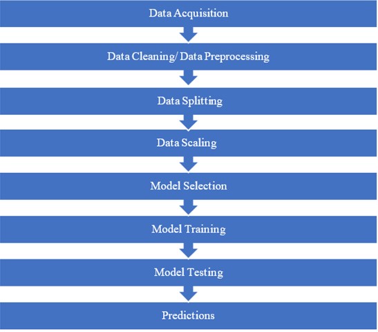
Table 2Parameter and values
Parameter | Values |
Pressure | Bar, 1 bar = 14.7 psi |
Inflow rate | 1 m3/sec |
Outflow rate | 1m3/sec |
Permeability | Millidarcy |
Length | 1 m |
Height | 1 m |
Width | 1 m |
Viscosity of water | 1 cp |
Table 2 presents the parameter values used in the problems discussed in this paper, while Table 3 shows the corresponding boundary conditions. The specific inflow and outflow rates used were both 1 m3/sec. The focus of the study was on investigating changes in pressure, which was specified at the corners of a simple 2D flow model using injection and production wells. The main objective was to solve equation 2 for pressure p over an arbitrary domain , subject to appropriate boundary conditions (either Neumann or Dirichlet) on boundary . The term represents a specified flow rate, while . The matrix can be a diagonal or a full cartesian tensor with a general form that can be expressed as:
The full tensor pressure equation is assumed to be elliptic such that . The tensor can be discontinuous across internal boundaries of ([25]).
Table 3Boundary condition
1 | –1 | |
0 1 | ||
0 1 |
3.2. Data collection for machine learning method
In this study, we utilized the Finite-volume approach to solve the elliptic PDE and gather data using MATLAB for various scenarios based on the problem stated in Section 3.1. We assumed the following while collecting data:
1) Permeability was assumed to be symmetrical and constant within each cell.
2) We placed an injection well at the origin and production wells at the points (±1, ±1).
3) No-flow conditions were specified at all other boundaries.
4) These boundary conditions resulted in the same flow as if we extended the five-spot well pattern to infinity in every direction. The flow in the five-spot is symmetric about both the coordinate axes.
5) We approximated the pressure pw with a cell-wise constant function and estimated across cell interfaces using a set of neighboring cell pressures to obtain Finite-volume methods.
3.3. Data preprocessing
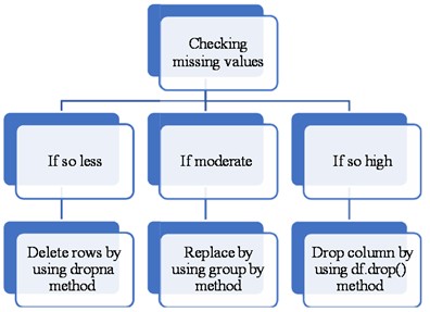
The preprocessing of data is a critical task for machine learning algorithms. It involves transforming raw data into usable and understandable data. Raw data may contain missing values or erroneous entries that could lead to errors in the model. Therefore, it is essential to clean the data before feeding it into a machine learning model. In this step, we check for any missing values and erroneous entries in the data collected from the series of cases simulated using the Finite-Volume Method (FVM) approach for training and testing. Fig. 5 displays the presence or absence of missing values in our dataset for the 8×8 grid. Additionally, Fig. 6 presents a conceptual workflow for handling missing values and verifying erroneous entries.
3.4. Data splitting
Dividing the dataset into training and testing sets is a crucial step in any machine learning approach. The data is divided into two subsets: the training data and the testing data. To perform data splitting, we can utilize the inbuilt sklearn library. In our study, we partitioned the dataset into 90 % for training data and 10 % for validation data. Additionally, we generated additional datasets for testing purposes to evaluate the performance of our model on previously unseen data.
3.5. Feature scaling
Data scientists often assume that their data follows a Gaussian (normal) distribution, which forms the basis of many machine learning models. Therefore, it is essential to convert the dataset into a normal distribution form. This is achieved by applying appropriate transformations to the dataset. To verify normality in the dataset, we can use a histogram or QQ plot. Feature scaling is a technique that standardizes the independent or dependent features of the data to a fixed range. If feature scaling is not applied, the machine learning algorithm may assign higher weights to greater values and lower weights to smaller values, regardless of their units. Feature scaling is performed during data preprocessing to handle data with varying units, magnitudes or values.
Fig. 5Checking for missing values in grid 8×8
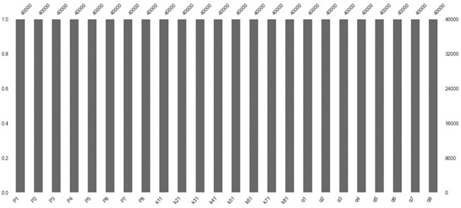
Fig. 6Workflow for Handling missing values
3.6. Model selection
Regression model in supervised machine learning is used to predict continues values. There are many types of regression models in machine learning. Selection of the model is mainly dependent upon the dataset. Seaborn, the visualization library of Python can be used to check the dependence of target variable on features. It requires a lot of experience to choose the model. The other method to select a model depends on the errors. This is an easy method. Lower the error, better the performance of the model. The names of the machine learning models on which we work in this paper are:
– Linear regression.
– Lasso regression.
– Support vector regression.
– Random forest regression.
– XG Boosting.
– Lightweight boosting.
– Decision tree regressor.
– Perceptron.
– ANN.
– CNN.
3.7. Machine learning model training
As discussed in the Data splitting section, data is split into two parts where training data used to train the model. After selecting the model, training data is used to find the relationship between the target variable and the features. Model tries to fit the data according to selected model. Then the model finds the relationship between features and target and stores it in a variable. Model training is done for all three models one by one.
3.8. Machine learning model testing
Relationship between target variable and the features found from model training is used to predict the target by using testing data. Then the target variable in testing data and the predicted values of target variable with help of testing features data are compared. The model is evaluated by finding the various type of error between above two data. To check the performance of the model three types of errors are useful:
– Mean absolute error.
– Mean squared error.
– Root mean squared error.
3.8.1. Mean absolute error
It is the mean of sum of Absolute errors. It can be expressed as the formula given below:
where – actual target value, – predicted target value, – number of data.
3.8.2. Mean squared error
It is the mean of sum of square of the errors. It can be expressed as the formula given below:
3.8.3. Root mean squared error
It is the square-root of the mean of sum of square of the errors. It can be expressed as the formula given below:
In this paper we will work mean absolute error and mean squared error.
4. Results
Next, we present the results of our machine learning approaches. Table 4 shows the architecture of CNN model for 2×8 grid, 8×8 grid, 32×32 grid and 64×64 grid dimensions. We used Relu. Activation function in hidden layers for all dimensions of grid and linear activation in output layers for all dimension of grid. For 2×8 grid, which means that grid has 2 layers in direction and 8 cells in direction, support vector regression model works best with a mean absolute error of 0.69. SVR works better than linear regression because it uses kernel function, so our model can work on non-linear datasets too. Kernel function which we used in the model is radial basis function (RBF). Without the hyper-tuning Decision tree regression model having an over-fitting problem on 2×8 Grid, we get very low errors in the training dataset of order 10-16 and we get extremely high errors on validation and testing datasets. Best Parameters which minimize over-fitting are max depth = 3, min samples leaf = 1, and min samples split = 2. We found thar our model for comparison in higher dimension grid gives larger errors.
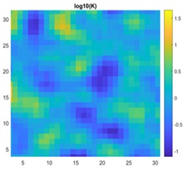
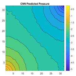
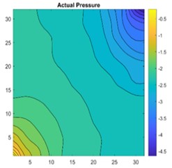
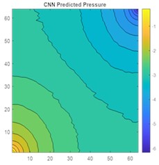
Fig. 7a) 2D view of permeability distribution using FVM, b) CNN predicted pressure, c) actual pressure using FVM and d) Lasso predicted pressure for 8×8 grid
4.1. Mean absolute and mean squared errors
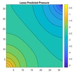
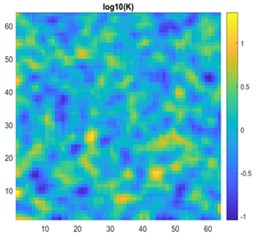
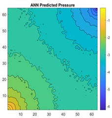
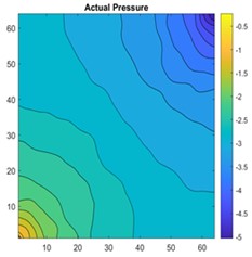
The results are compared for different models on grid dimensions of 2×8, 8×8, 32×32, and 64×64 using mean absolute errors (presented in Figs. 8-11) and mean squared errors (presented in Figs. 11-15). Results indicated that the models performed well, and there was not a significant difference in mean absolute error between validation and testing. The 2D results obtained from machine learning models are compared to actual pressure on 8×8, 32×32, and 64×64 grids (shown in Fig. 7 and Fig. 16-17). The (a) part shows input permeability, the (c) part shows the actual pressure output obtained from the Finite-Volume approach, and the (b) and (d) parts show the pressure predicted through machine learning model.
Table 4Architecture of CNN model
Grid | No. of hidden layers | Activation | Kernel size | kernel_regularizer | Learning rate | |
Hidden layer | Output layers | |||||
2×8 | 5 (4 CNN layers (filters=512,256, 128,64) and 1 Dense layers (filters = 32)) | Relu | Linear | 3 | L2 Regularizer with an alpha value of .01 at the Dense Layer | 1e-06 |
8×8 | 6 (5 CNN layers (filters=1024,512,256 ,128,64) and 1 Dense layers (filters = 32)) | Relu | Linear | 3 | L2 Regularizer with an alpha value of .01 at the last layer of CNN layers | 1e-03 |
32×32 | 4 (3 CNN layers (filters = 256, 128, 64) and 1 Dense layers) | Relu | Linear | 3 | L2 Regularizer with an alpha value of .01 at the last layer of CNN layers | 1e-06 |
64×64 | 3 (2 CNN layers (filters = 128, 64) and 1 Dense layers (filters = 32)) | Relu | Linear | 3 | L2 Regularizer with an alpha value of .01 at the last layer of CNN layers | 1e-03 |
Fig. 8Mean absolute error on 2×8 grid
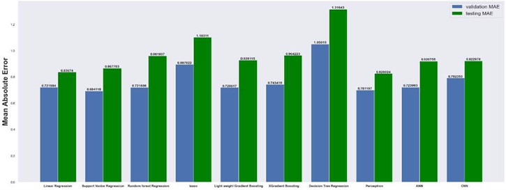
Fig. 9Mean absolute error on 8×8 grid
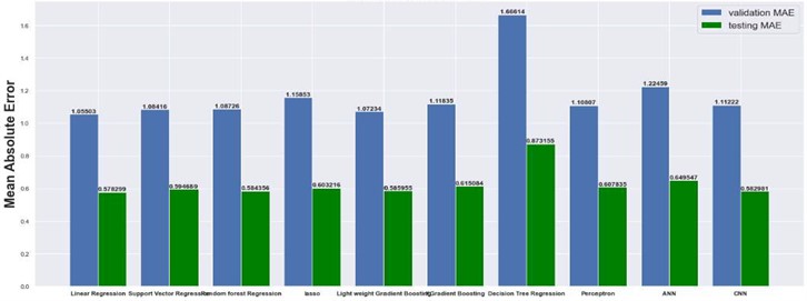
Fig. 10Mean absolute error on 32×32 grid
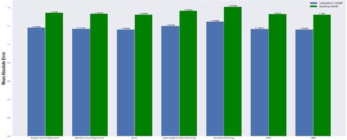
Fig. 11Mean absolute error on 64×64 grid
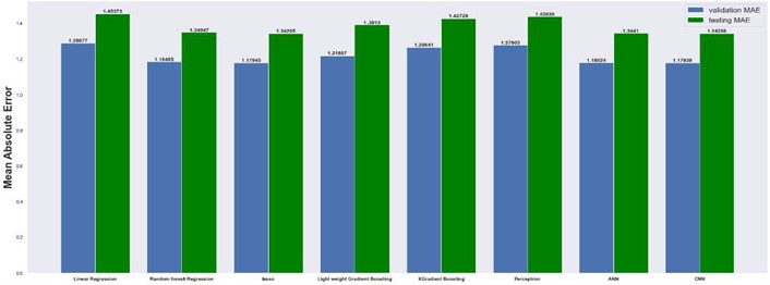
Fig. 12Mean squared error on 2×8 grid
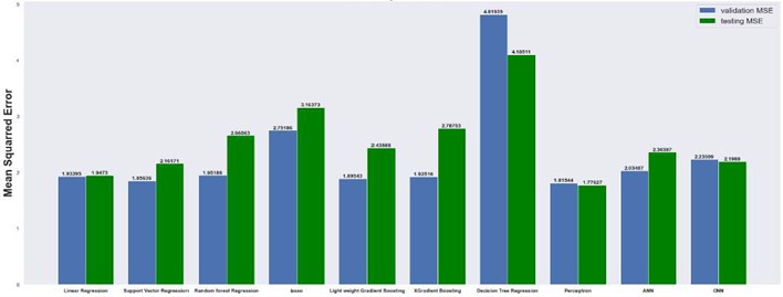
Fig. 13Mean squared error on 8×8 grid
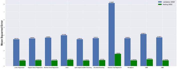
Fig. 14Mean squared error on 32×32 grid
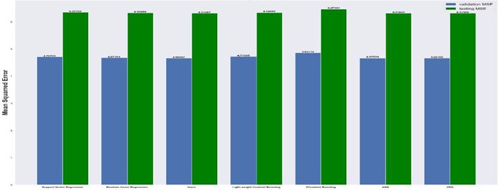
Fig. 15Mean squared error on 64×64 grid
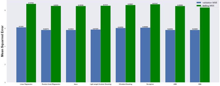
Fig. 16a) 2D view of permeability distribution, b) CNN predicted pressure, c) actual pressure, d) lasso predicted pressure for 32×32 grid
a)
b)
c)
d)
Fig. 17a) 2D view of permeability distribution, b) ANN predicted pressure, c) actual pressure, d) CNN predicted pressure for 64×64 grid
a)
b)
c)
d)
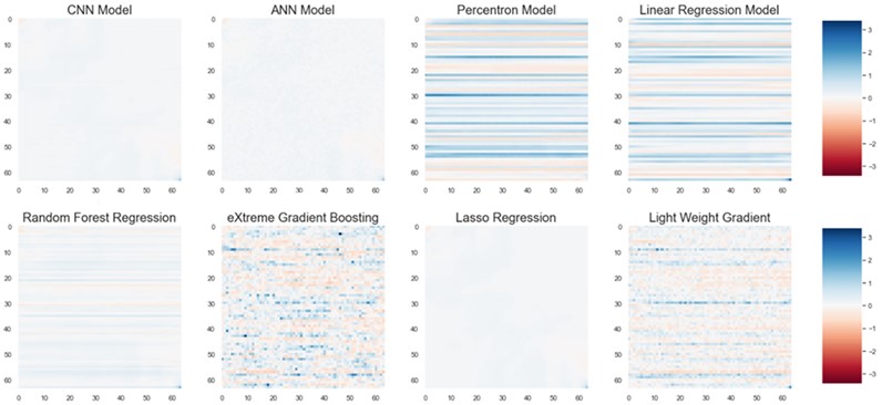
4.2. Residual errors
To verify our result, we used residual plot. The residual plot shows the difference between the observed response and the fitted response values. Simply if our model can predict actual pressure then it shows zero difference, in our plot this can be shown by white color. The residual plots are shown for 8×8 grid, 32×32 and 64×64 grids for different methods that are presented in Figs. 18-21.
Fig. 18Residual plot for CNN, ANN, random forest and decision tree regression for 8×8 on a grid
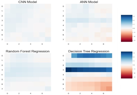
Fig. 19Residual plot for perceptron, support vector regression, linear regression, Lasso regression, light weight gradient, eXtreme Gradient Boosting on an 8×8 grid
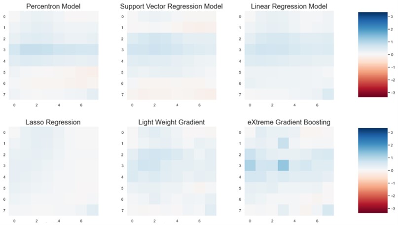
Fig. 20Residual plot for a) random forest, b) eXtreme gradient boosting, c) Lasso regression, d) CNN model, e) ANN Model, f) support vector regression model for 32×32 grid
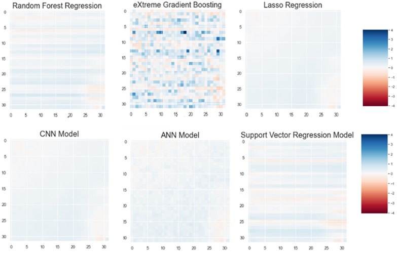
Fig. 21Residual plot for CNN, ANN, perceptron, linear regression, random forest regression, eXtreme gradient boosting, Lasso regression, light weight gradient boosting for 64×64 grid
5. Conclusions
The paper begins by generating a material balance equation and defining a finite volume approach mathematically for Darcy's equation. To predict pressure variation in a reservoir based on permeability variation in different grid sizes, several machine learning approach have been tested. Ten different machine learning models, including linear regression, support vector regression, random forest regression, lasso regression, light weight gradient boosting, extreme gradient boosting, decision tree regression, perceptron, artificial neural network (ANN), and convolutional neural network (CNN) were used to predict pressure. The analysis shows that CNN, linear regression, and lasso regression had the lowest mean absolute error (MAE) and mean squared error (MSE) values, while the decision tree regression model had the highest error. The CNN model demonstrated the best performance on the validation dataset for most grid dimensions, and both the CNN and ANN models performed well on a 64×64 grid. In conclusion, the lower the error values, the better the model performance, and the CNN and ANN models demonstrated good performance for this particular prediction task.
References
-
A. M. Tartakovsky, C. Ortiz Marrero, Paris Perdikaris, and Guzel D. Tartakovsky, “Physics informed deep neural networks for learning parameters and constitutive relationships in subsurface flow problems,” Pacific Northwest National Laboratory, 2020.
-
H. Wu and R. Qiao, “Physics-constrained deep learning for data assimilation of subsurface transport,” Energy and AI, Vol. 3, p. 100044, Mar. 2021, https://doi.org/10.1016/j.egyai.2020.100044
-
R. M. Maxwell, L. E. Condon, and P. Melchior, “A physics-informed, machine learning emulator of a 2D surface water model: what temporal networks and simulation-based inference can help us learn about hydrologic processes,” Water, Vol. 13, No. 24, p. 3633, Dec. 2021, https://doi.org/10.3390/w13243633
-
H. Chang and D. Zhang, “Machine learning subsurface flow equations from data,” Computational Geosciences, Vol. 23, No. 5, pp. 895–910, Oct. 2019, https://doi.org/10.1007/s10596-019-09847-2
-
J. Li, D. Zhang, N. Wang, and H. Chang, “Deep learning of two-phase flow in porous media via theory-guided neural networks,” SPE Journal, Vol. 27, No. 2, pp. 1176–1194, Apr. 2022, https://doi.org/10.2118/208602-pa
-
C. El Morr, M. Jammal, H. Ali-Hassan, and W. Ei-Hallak, International Series in Operations Research and Management Science. Cham: Springer International Publishing, 2022, https://doi.org/10.1007/978-3-031-16990-8
-
R. Tibshirani, “Regression shrinkage and selection via the lasso,” Journal of the Royal Statistical Society: Series B (Methodological), Vol. 58, No. 1, pp. 267–288, Jan. 1996, https://doi.org/10.1111/j.2517-6161.1996.tb02080.x
-
M. A. Hearst, S. T. Dumais, E. Osuna, J. Platt, and B. Scholkopf, “Support vector machines,” IEEE Intelligent Systems and their Applications, Vol. 13, No. 4, pp. 18–28, Jul. 1998, https://doi.org/10.1109/5254.708428
-
L. Breiman, “Random forests,” Machine Learning, Vol. 45, No. 1, pp. 5–32, 2001, https://doi.org/10.1023/a:1010933404324
-
C.-Y. J. Peng, K. L. Lee, and G. M. Ingersoll, “An introduction to logistic regression analysis and reporting,” The Journal of Educational Research, Vol. 96, No. 1, pp. 3–14, Sep. 2002, https://doi.org/10.1080/00220670209598786
-
G. Guo, H. Wang, D. Bell, Y. Bi, and K. Greer, “KNN model-based approach in classification,” in On the Move to Meaningful Internet Systems 2003: CoopIS, DOA, and ODBASE, pp. 986–996, 2003, https://doi.org/10.1007/978-3-540-39964-3_62
-
S. Mishra et al., “Principal component analysis,” International Journal of Livestock Research, 2017, https://doi.org/10.5455/ijlr.20170415115235
-
H. Andrews and C. Patterson, “Singular value decomposition (SVD) image coding,” IEEE Transactions on Communications, Vol. 24, No. 4, pp. 425–432, Apr. 1976, https://doi.org/10.1109/tcom.1976.1093309
-
F. Rosenblatt, “The perceptron: a probabilistic model for information storage and organization in the brain,” Psychological Review, Vol. 65, No. 6, pp. 386–408, 1958, https://doi.org/10.1037/h0042519
-
Y. Lecun, L. Bottou, Y. Bengio, and P. Haffner, “Gradient-based learning applied to document recognition,” Proceedings of the IEEE, Vol. 86, No. 11, pp. 2278–2324, 1998, https://doi.org/10.1109/5.726791
-
K. Simonyan and A. Zisserman, “Very deep convolutional networks for large-scale image recognition,” arXiv e-prints, p. arXiv:1409.1556, 2014, https://doi.org/10.48550/arxiv.1409.1556
-
C. Szegedy et al., “Going deeper with convolutions,” in 2015 IEEE Conference on Computer Vision and Pattern Recognition (CVPR), pp. 1–9, Jun. 2015, https://doi.org/10.1109/cvpr.2015.7298594
-
K. Fukushima, “Neocognitron: A self-organizing neural network model for a mechanism of pattern recognition unaffected by shift in position,” Biological Cybernetics, Vol. 36, No. 4, pp. 193–202, Apr. 1980, https://doi.org/10.1007/bf00344251
-
A. Krizhevsky, I. Sutskever, and G. E. Hinton, “ImageNet classification with deep convolutional neural networks,” Communications of the ACM, Vol. 60, No. 6, pp. 84–90, May 2017, https://doi.org/10.1145/3065386
-
X. Zhang, X. Zhou, M. Lin, and J. Sun, “ShuffleNet: an extremely efficient convolutional neural network for mobile devices,” in 2018 IEEE/CVF Conference on Computer Vision and Pattern Recognition (CVPR), pp. 6848–6856, Jun. 2018, https://doi.org/10.1109/cvpr.2018.00716
-
G. Huang, Z. Liu, L. van der Maaten, and K. Q. Weinberger, “Densely connected convolutional networks,” in 2017 IEEE Conference on Computer Vision and Pattern Recognition (CVPR), pp. 2261–2269, Jul. 2017, https://doi.org/10.1109/cvpr.2017.243
-
A. Paszke, A. Chaurasia, S. Kim, and E. Culurciello, “ENet: a deep neural network architecture for real-time semantic segmentation,” arXiv, 2016, https://doi.org/10.48550/arxiv.1606.02147
-
J. E. Aarnes, T. Gimse, and K. Lie, “An introduction to the numerics of flow in porous media using Matlab,” in Geometric Modelling, Numerical Simulation, and Optimization, 2007, https://doi.org/10.1007/978-3-540-68783-2_9
-
M. Bagheri et al., “Data conditioning and forecasting methodology using machine learning on production data for a well pad,” in Offshore Technology Conference, May 2020, https://doi.org/10.4043/30854-ms
-
M. Pal, P. Makauskas, M. Ragulskis, and D. Guerillot, “Neural solution to elliptic PDE with discontinuous coefficients for flow in porous media,” ECMOR 2022, 2022.
-
J. Vink, “Computing challenges in oil and gas field simulation,” in XI International Workshop on Advanced Computing and Analysis Techniques in Physics Research, 2009.
-
M. Pal, P. Makauskas, P. Saxena, and P. Patil, “The neural upscaling method for single-phase flow in porous medium,” in ECMOR 2022, Vol. 2022, No. 1, pp. 1–13, 2022, https://doi.org/10.3997/2214-4609.202244021
-
M. Pal, P. Makauskas, M. Ragulskis, and D. Guerillot, “Neural solution to elliptic PDE with discontinuous coefficients for flow in porous media,” in ECMOR 2022, Vol. 2022, No. 1, pp. 1–17, 2022, https://doi.org/10.3997/2214-4609.202244023
-
M. Pal, “Families of flux-continuous finite-volume schemes,” Ph.D. Thesis, Swansea University, 2007.
About this article

The authors have not disclosed any funding.
The datasets generated during and/or analyzed during the current study are available from the corresponding author on reasonable request.
Shankar Lal worked on modelling, preparing draft and reviews. Neetish Kumar worked on draft review and conceptualization, Vilte Karaliute worked on draft reviews and generating proper images, Mayur Pal provided overall guidance, conceptualization and draft writing.
The authors declare that they have no conflict of interest.
