Abstract
Loose particles inside components can be threats to their reliabilities. Automatic identification of loose particles’ material has great significance for finding the source of them. Machine learning methods based on hand-craft features have been widely applied on this problem. As deep learning has made success on various domains, based on PIND (particle impact noise detection) test, a method using spectrograms and CNN (convolutional neural network) is proposed in this paper. First, signals of loose particles including different material are collected by experiments. Then signals are converted to spectrograms. Finally, spectrograms are input to CNN for training and classification. Experiments show that the method can achieve 96 % accuracy on identifying five types of loose particles and has values of practically use.
1. Introduction
The existence of loose particles is one of the main threats to the reliability of aerospace components, which can lead to fatal accidents. For example, a small piece of iron sheet can move to bared wires and cause short circuits. Loose particles can be brought in while producing the components and it’s hard to clear them out absolutely.
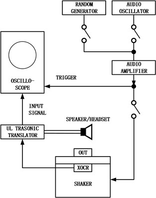
Detecting the loose particles before the components are put into use is one way to improve. Particle impact noise detection (PIND) test is a major method for detecting the presence of loose particles left inside components. Following MIL-STD-202G standard [1], the structure of PIND test is as shown in Fig. 1. Its process can be described as follows:
1) Put the component to be tested on the shaker or turntable, and attach the acoustic sensor on it.
2) The shaker produces impact and vibration, which makes loose particles inside the component free and impact with the component.
3) The impact produces acoustic signal, which is collected by the acoustic sensor. The sensor can converts the acousitc signal to electrical signal, and then output it to oscilloscope and speaker.
4) The oscilloscope can show visible waveform and the speaker can provide audible sound. The operator can use this information to determine the presence and classification of loose particles.
Besides detecting the presence of loose particles, identifying the material is also necessary. It can help find the source of loose particles and can be helpful for reducing their generation. Material identification is actually a classification problem. Traditional methods usually use machine learning to solve the problem, the usual process is extracting features from acoustic signals firstly and training classifiers then. Shujuan Wang [2] proposed a LVQ (Learning Vector Quantization)-based method which uses energy distribution vectors in wavelet domain. Long Zhang [3] compared the wavelet Fisher discriminant with AR model and LVQ neural networks and proves that the wavelet Fisher discriminant is better than others. JinBao Chen [4] uses MFCC (Mel Frequency Cepstrum Coefficient) feature to train HMM (Hidden Markov Model), achieving 91 % accuracy on 4 types of material. Meng [5] combines MFCC with other features in time and frequency domain to train SVM (Support Vector Machine) model, achieving 98 % on 3 types of material. For these methods, the performance of identification is determined by whether the features can represent information of material completely and whether the classifier can map features to classes accurately. However, the hand-craft features may be hard to characterize the material information of original signals accurately, especially for complex signals with noisy signals.
Fig. 1The structure of PIND test
In order to overcome the disadvantages of hand-craft features, we need an end-to-end algorithm which can gives the identification result directly, which means both features extraction and classification are finished by it. Recent work on speech recognition has shown good performance [6, 7]. Cummins N’s work [6] on speech emotion recognition has shown that using pre-trained CNN (convolutional neural network) to extract features from spectrograms is robust for noisy signals. Li P. [7] proposed an attention pooling based CNN which also receives a spectrogram as input, having shown excellent performance. As deep learning has not been applied on the problem of loose particles’ material identification, motivated by these works, a method using spectrogram and CNN is proposed. In this way, extracting features manually can be avoided. Instead, the network searches appropriate features from the spectrogram automatically. Experiments prove that deep learning method outperforms existing methods.
2. Method
2.1. Task description
Identification of loose particles aims to predict their types artificially or automatically according to PIND signals collected by the detection system. The component which may have latent loose particles is put on the device, and by adding vibration acoustic signals are collected. To avoid collecting useless noise signals, a trigger thresh is set and we only record the signal when it reaches the thresh. Components having known loose particles are used for experiments, thus we can collect signals with known labels. Our method aims to train a model to classify the signals datasets.
2.2. Identification based on CNN
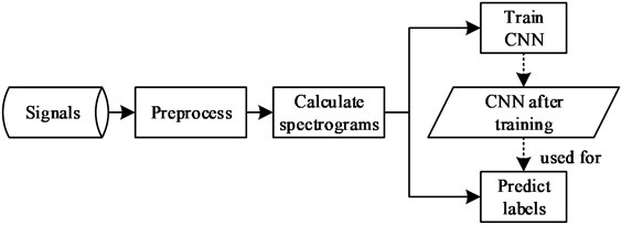
The process of material identification using deep learning includes follows: 1) Preprocess original signals to reduce noises. 2) Calculate spectrograms of denoised signals. 3) Input spectrograms with their material labels to an end-to-end CNN to train the model. 4) Use the trained model to predict test signals’ material types. It can be shown as Fig. 2.
Fig. 2Process of proposed material identification method
2.2.1. Spectrograms calculation
Before calculating spectrograms, DB4 wavelet denoising is applied on signals as preprocessing. Related work in paper [8] has proved its effectiveness. As a CNN receives images as input, spectrograms are firstly calculated.
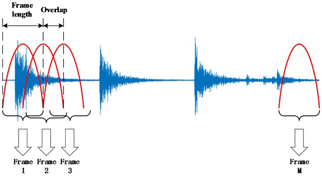
Firstly, the signal is divided into several frames with the same length, and then a sequence of hamming windows are applied to these frames. Hamming window can be calculated as Eq. (1):
where refers to the length of windows and should be same with frame length. Dot the signal by window to acquire the output.
To avoid information missing at both ends of hamming window, there exists overlap between neighboring frames. Usually overlap is set to 1/3-1/2 of frame length and here we use half (0.5 ms). The process of applying windows is shown in Fig. 3.
Fig. 3Divide frames and apply hamming windows
For each frame with length of , we calculate the DFT (discrete Fourier transform) result as Eq. (2):
Assuming that the number of frames in one signal is , then we concate all the DFT results (each is a vector) and get a matrix as Eq. (3):
In ways similar to pseudo-color processing, the matrix can be mapped to an colored image. Thus, a spectrogram is calculated.
2.2.2. Spectrograms of loose particle signals
An example of loose particle signal with its spectrogram is shown as Fig. 4. As is shown in Fig. 4(b), the pulse signals around 0-20 ms, 45-60 ms, 65-80 ms, 85-95 ms have common features that the power around 50 kHz is especially high, and their shapes are also similar.
Fig. 4An example of loose particle signal with its spectrogram
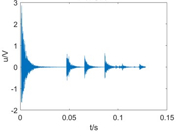
a) Signal
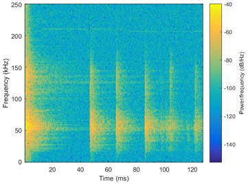
b) Spectrogram
Fig. 5 shows 2 spectrograms of different material’s loose particle signals. Epoxy’s frequency mainly focus on 50 kHz, while wire’s frequency has a higher range. On the one hand, there exists difference among spectrogram of different material’s loose particle signals. On the other hand, pulses in the same spectrogram are similar in peak position and envelope. So spectrograms are able to represent the information of material, and using spectrograms as the input of CNN is a available way to achieve automatic identification.
Fig. 5Spectrograms of different material’s PIND signals
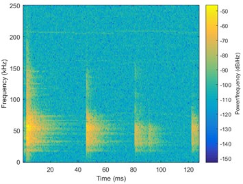
a) Epoxy
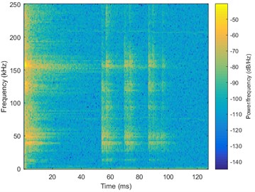
b) Wire
2.2.3. CNN architecture
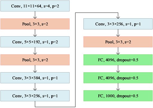
Based on AlexNet [9], a similar CNN architecture is used for classifying the spectrograms. The architecture is shown as Fig. 6. For convolution layer, 11×11×64 denotes height × width × channel of kernels. For pooling layer, 3×3 denotes height × width of kernels. Stride and padding size is denoted by s and p (where 0 is omitted). Number in fully connected layer shows the number of nodes, and dropout percentage is also given. Besides, in order to accelerate the training process, a pre-trained model trained on Image Net database is used. Though there are 1000 class in this model, it can still be applied on 5-class problem in later experiments.
Fig. 6Network architecture
3. Experiments
For experiments, a dataset of loose particle signals are collected, including 4794 sample signals. There are 5 different types of loose particles, including tin, epoxy, tinsel, aluminum and wire. Considering mass of loose particles are usually not stable, loose particles range from 0.1 mg-4 mg are used. The dataset is divided into 2 part, 1/4 is randomly chosen for testing and others are for training. For spectrograms calculation, frame length is 1 ms and DFT length is 256.
3.1. Network training and testing
A pre-trained model trained on Image Net is used as initial model to accelerate the training process. Optimization method is gradient descent method, and learning rate is 0.003. Use cross entropy function as loss function. After enough iteration, accuracy on the training dataset is close to 100 %, and accuracy on the testing dataset is close to 96 %.
3.2. Loose particles identification experiments
We tested our model on loose particle signals datasets. Table 1shows the identification result in form of confusion matrix. The material in the left column denotes true labels, while the top row denotes predictions. The number at the intersect represent the amount. Though the identification accuracy on aluminum is obviously worse than other materials, the overall accuracy on the whole test datasets still achieves 96.16 %.
Table 2 shows the results compared with other methods. As there is no open dataset of loose particle signals, results of [2-4] in the table is given by corresponding papers, and others come from experiments on our datasets. The proposed method outperforms [2-4] with more classes and shorter signals, and outperforms all methods with higher accuracy.
Table 1Identification result (confusion matrix) on testing dataset
True | Predict | |||||
Tin | Epoxy | Tinsel | Al | Wire | Accuracy | |
Tin | 167 | 3 | 1 | 2 | 0 | 96.5 % |
Epoxy | 4 | 471 | 1 | 2 | 3 | 97.9 % |
Tinsel | 2 | 3 | 235 | 4 | 1 | 95.9 % |
Al | 4 | 4 | 2 | 186 | 3 | 93.4 % |
Wire | 0 | 4 | 0 | 2 | 95 | 94.0 % |
Table 2Method comparison
Method | [2] | [3] | [4] | [5] | Ours |
Number of types | 4 | 3 | 4 | 5 | 5 |
Particle mass / mg | 0.5-2.5 | 0.5-6 | 1-4 | 0.1-4 | 0.1-4 |
Signal length / s | 1 | 5 | 5 | 0.128 | 0.128 |
Accuracy / % | 83 | 87 | 91 | 92 | 96 |
4. Conclusions
Automatic material identification of loose particles has vital research value for improving the reliability and stability of components. Related researches before mostly used hand-craft and machine learning methods. As deep learning and spectrograms are widely used in speech recognition domain, this paper proposes to apply CNN with spectrograms on the loose particles’ material identification task. Experiments prove that the proposed method achieves higher accuracy and it is useful in practical production. The network structure used in this paper still need to be improved, and learning features from the signal directly is also an important trend in future research.
References
-
MIL-STD-202G, Test Method Standard Electronic and Electrical Component Parts. American Department of Defense, 2002.
-
Wang S., Chen R., Zhang L., et al. Detection and material identification of loose particles inside the aerospace power supply via stochastic resonance and LVQ network. Transactions of the Institute of Measurement and Control, Vol. 34, Issue 8, 2012, p. 947-955.
-
Zhang L., Li K., Wang S., et al. Loose particle classification using a new wavelet fisher discriminant method. International Symposium on Neural Networks, Berlin, Heidelberg, 2013, p. 582-593.
-
Chen J. Signal pattern recognition and confidence evaluation for loose particle detection of sealed electronic devices. Harbin Institute of Technology, 2015.
-
Meng C., Li Y., et al. Signal recognition of loose particles inside aerobat based on support vector machine. Journal of Beijing University of Aeronautics and Astronautics, Vol. 46, Issue 3, 2020, p. 488-495.
-
Cummins N., Amiriparian S., Hagerer G., et al. An image-based deep spectrum feature representation for the recognition of emotional speech. Proceedings of the 25th ACM International Conference on Multimedia, 2017, p. 478-484.
-
Li P., Song Y., Mc Loughlin I. V., et al. An attention pooling based representation learning method for speech emotion recognition. 19th Annual Conference of the International-Speech-Communication-Association, 2018, p. 3087-3091.
-
Wu Y., Wang S., Wang S. Research on wavelet threshold de-noising method of remainder detection for stand-alone electronic equipments in satellite. 1st International Conference on Pervasive Computing, Signal Processing and Applications. 2010, p. 1013-1017.
-
Krizhevsky Alex, et al. Image net classification with deep convolutional neural networks. Advances in Neural Information Processing Systems, Vol. 25, 2012, p. 1097-1105.
About this article

This work is partly supported by NSFC under No. 91748201.
