Abstract
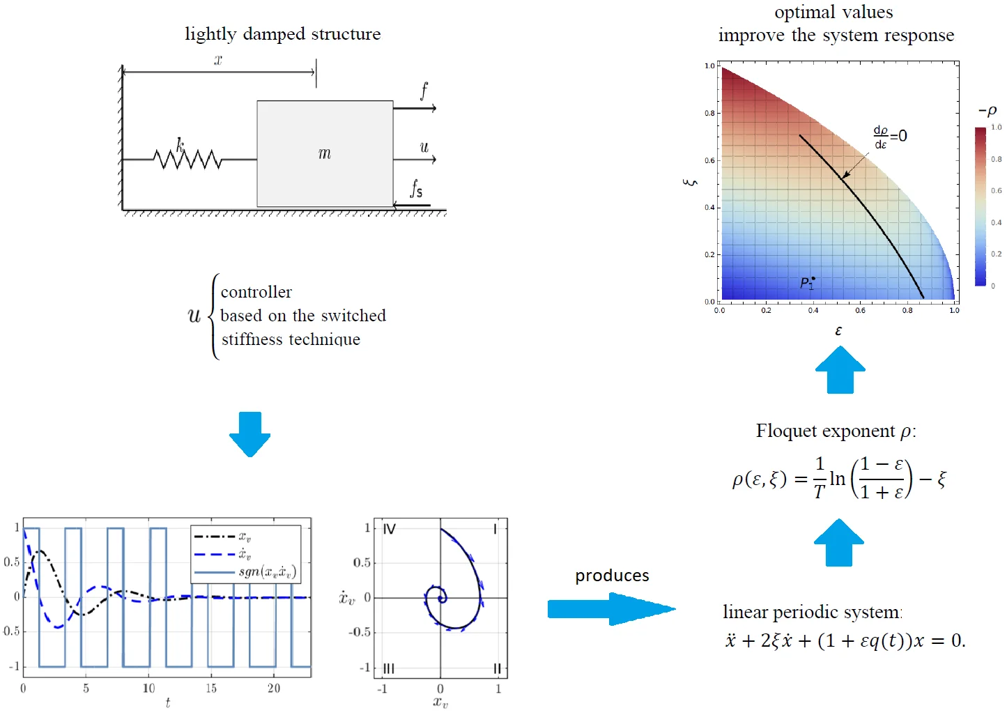
An active damping controller based on the switched stiffness technique is developed and applied to vibration mitigation in a lightly damped structure. The controller either increases or decreases the system stiffness according to a state-dependent rule. A novel stability analysis based on the Floquet theory is proposed and employed to analyze the mathematical model of a one-degree-of-freedom system where the friction forces are taken into account. This novel analysis allows us to prove the exponential stability of the system origin, to establish a tuning procedure for the controller gain, to solve an optimization problem and to show the controller robustness against parameter uncertainties. Experimental verification is conducted to validate the effectiveness of the controller, and it is shown that the controller is feasible for vibration control problems.
Highlights
- State-dependent control law produces a periodic response
- The period of the system response can be calculated analytically
- A lightly damped system is stabilized and optimal values can be obtained for the controller
1. Introduction
The stiffness modification is a well-known semi-active control technique for the vibration mitigation in structures and it was first introduced by Chen [1] and studied extensively by Onoda [2, 3]. This technique is achieved by semi-active devices whose stiffness is changed according to a state-dependent control rule. The most employed rule corresponds to switch the device between a maximum and minimum stiffness value, i.e., the semi-active device performs a switched stiffness control strategy [4].
Over the years, an enormous amount of research has been devoted to the implementation and experimental verification of the switched stiffness technique through developing semi-active stiffness devices. For instance, in [2] a piezoelectric actuator is implemented, while in [5] a spring with a mechanical arrangement is used to switch the stiffness. In [6] a valve is used as a semi-active device, while in [7] an electromagnetic device is developed, and recently a magnetostrictive transducer is developed in [8], to name a few.
Although a considerable body of research has been done in developing semi-active stiffness devices, few attempts have been made to investigate the relation between the device parameters and their performance for vibration control in structures. Pioneer work was done in [9] where it is performed a characterization of the parameters of the semi-active devices by introducing a dimensionless parameter that relates the maximum and minimum stiffness. In the same work, it is found the optimal parameter value for which the damped response is improved. However, in practical terms, such optimal value cannot be handled by the switched stiffness devices. Consequently, the limitations of the switched stiffness technique are increasingly apparent.
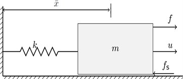
This study aims to extend the applicability of the switched stiffness technique by considering that the control action is applied actively via an actuator. For illustrative purposes, the active damping of a one-degree-of-freedom system is analyzed considering the free vibration case. That is, consider the physical realization of the one-degree-of-freedom system given by the mass-spring system shown in Fig. 1, then the switched stiffness technique is applied actively by the force defined by , where is the controller gain. The control action increases or decreases the system stiffness at the specific instants.
Thereupon, our main goal is to determine the effectiveness of active control for vibration mitigation in structures considering a switched stiffness technique. Also, we conduct experimental verification of the approach.
Fig. 1Actuated mass-spring system with friction
This paper is organized as follows. The Section 2 is dedicated to problem formulation and some fundamental ideas underlying the main problem are presented, while Section 3 details our theoretical findings based on the application of the Floquet theorem, to clarify our results, background information about the theory is briefed in the appendix. The Section 4 provides numerical and experimental results that support our findings and some final comments on the results are given in the conclusion Section 5.
2. Problem formulation
Consider the one-degree-of-freedom system given by the lightly damped mass-spring system shown in Fig. 1. The body slides on a surface with friction, and we assume that the dissipative phenomenon due to the friction force can be approximated by a linear viscous damping force , where is the damping coefficient. In practice, this assumption provides mathematical tractability and simplicity, besides the damping coefficient can be estimated by well-known techniques [10, 11]. The characterization of the involved dissipative forces as a linear viscous damping force is a proven approximation and is feasible for a neighborhood around the origin. Accordingly, the mathematical model of the system is given by:
where is the mass, is the stiffness, is the control law, the prime denotes differentiation with respect to time and are non-zero initial conditions. The control law is defined by:
where is the controller gain and denotes the standard sign function.
Let us define the non-dimensional parameters: the damping ratio , the natural frequency and . Thus, the time scale and the variable change , where is a constant, transform Eq. (1) into:
where the dots denote differentiation with respect to time , the initial conditions are reduced to and the tuning parameter is defined by , hence, the controller gain is given by:
When the viscous damping is not present, Eq. (3) is known as the Reid equation which has been used to describe the hysteretic damping occurred intrinsically in materials [12, 13]. Therefore, it is said that the switched stiffness technique induces a nonlinear dissipative phenomenon related to the hysteretic damping [14, 15]. For the analysis of this equation, several nonlinear analysis techniques have been broadly applied. For instance, in [14] the solution is approximated by the harmonic balance technique and its stability is determined by the variational equation, in [16] an extended analysis is done using perturbation techniques and the multi-degree-of-freedom case is studied in [17], while in [15, 18] a piecewise analytic approach is carried out, in [19] the phase plane method is developed and applied and [9] applies an approximation technique based on method of variation of parameters. A novel approach using linear techniques was also developed in [20].
From Eq. (3) written as state space model:
we deduce that the origin is an isolated equilibrium point, and the existence and uniqueness of the solution of Eq. (5) are guaranteed because the function satisfies the Lipschitz condition, it is bounded and piecewise continuous at and it admits a limited number of finite discontinuities [21].
In general, the semi-active control technique posses inherent stability as it is pointed out in [22]. Notwithstanding, for Eq. (3), the main question is about under what circumstances of the parameters its origin is stable. The stability of the origin can be established by the Lyapunov theorem as follows.
Consider the candidate Lyapunov function , then, its derivative along the trajectories of Eq. (5) yields:
which is negative semi-defined, then by the Lyapunov theorem the trivial solution of Eq. (3) is stable. However, applying the Young inequality, , to Eq. (6) yields:
where for and , the function is negative defined and the origin is asymptotically stable.
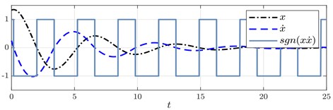
From the above result, it is shown that the Lyapunov analysis delimits the parameter range to ensure asymptotic stability. However, in general, there is not a procedure to choose an appropriated tuning parameter neither its optimum value, given a prescribed performance index. To illustrate this issue, consider the numerical solutions of Eq. (3) plotted in Fig. 2 for different values of the tuning parameter , along with the corresponding switching functions. From Fig. 2 we deduce several facts: first, the trajectories converge to zero as it was proved by Lyapunov analysis; second, the settling time of the response in the second case is shorter than the first case. Accordingly, a tuning methodology must be devised.
In Fig. 2, one more remarkable fact takes place, the switching function seems to behave periodically in time, at this point it is important to point out that we claim that the sign function of the product behaves periodically in time. This fact allows us to perform a stability analysis treating Eq. (3) as a linear periodic equation instead of a nonlinear differential equation. The principal advantage of doing this is that for linear systems several well-known mathematical tools can be employed instead of nonlinear approximation techniques. The main mathematical tool for periodic linear systems is the Floquet theory which for reference is briefed in the appendix to clarify our findings. In the following sections, the application of the Floquet theory shall allow us to prove the exponential stability of the origin, to establish a tuning procedure for the controller gain, to solve an optimization problem and to prove the controller robustness.
Fig. 2Numerical solutions of Eq. (3) with initial conditions (x0,x˙0)=(1.25,0.25): a) when ξ=0.15 and ε=0.1 and b) when ξ=0.15 and ε=0.45
a)
b)
3. Main results
The damped Reid equation Eq. (3), illustrates the case when the dissipative forces, which are ubiquitous in real-world systems, are taken into account. In this work, they are characterized and quantified by a viscous damping force, this assumption is feasible for a neighborhood around the origin [23]. We recall that in the absence of damping, Eq. (3) is reduced to the well-known Reid equation which has been broadly studied employing nonlinear analysis techniques, such studies in some cases are cumbersome and approximated.
We apply the Floquet theory to analyze the damped Reid equation. This approach is novel and simple, and it provides analytic results without employing approximations.
To apply the Floquet theory, it is necessary to rewrite the nonlinear differential equation Eq. (3) as a linear periodic differential equation, that is, we must prove that the function has a fixed period which must be independent of the initial conditions.
Recall that Fig. 2 suggests that switching function behaves periodically in time. In order to corroborate this fact, the set of arbitrary initial conditions of Eq. (3) are nondimensionalized and split into two sets in the following way: if and then the nondimensionalized initial conditions along with Eq. (3) allow us to define the initial position problem, while if and then the nondimensionalized initial conditions along with Eq. (3) defined the initial velocity problem. In this manner, we define a set of linearly independent initial conditions.
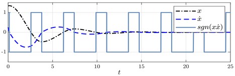
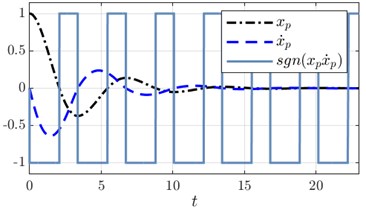
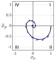
For the initial position and velocity problem above defined, their solutions and , along with the corresponding switching functions are plotted in Fig. 3(a) and Fig. 3(c) respectively. The plots reveal two remarkable facts: in both cases, the switching function behaves periodically in time as we expected and its period is fixed, and the second is that solutions approach asymptotically to the trivial solution with the same and fixed period. In this case the system described by Eq. (3) is said to be an asymptotically isochronous system, for a rigorous definition and examples see [24]. To prove the periodicity of the function, we must provide an analytic expression for the period by calculating the switching instants of the solutions as follows.
Fig. 3Numerical solutions Eq. (3) when ξ=0.25 and ε=0.15: a) solution for the initial velocity problem and its phase portrait b), c) solution for the initial position problem and its phase portrait d)
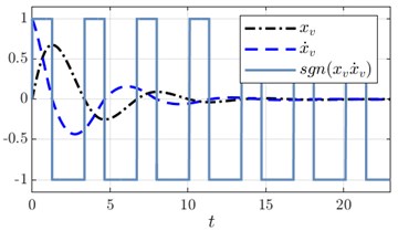
a)

b)
c)
d)
3.1. Periodicity
The phase portraits of the corresponding solutions and are plotted in Fig. 3(b) and Fig. 3(d) respectively. To calculate the switching instants , we examine both solutions at each quadrant of their respective phase portraits, where the function is well-defined, and hence, Eq. (3) is solvable and has analytic solutions.
3.1.1. Initial velocity problem
For the initial velocity problem the quadrants are named as in Fig. 3(b). At each quadrant we have the following:
I. At the first quadrant , then Eq. (3) is reduced to:
under the initial conditions . Its characteristic polynomial is whose roots are for a oscillatory response , then, , where . Thus, the solution is given by , where and are found applying the initial conditions, that is, the solution is and its derivative . At the first switching instant we have i.e, then and yields .
II. At second quadrant the relation holds, then Eq. (3) yields:
where . The roots of the characteristic polynomial are complex if , thus where . Then, the solution is , where and are integration constants applying the initial conditions, the solution is and its derivative yields . At the switching instant we have , that is, then and yields .
III. At the third quadrant , then Eq. (3) is reduced to with the initial conditions . The solution and its derivative are given by and respectively. At we have , that is, , and yields .
IV. In the last quadrant , then under the initial conditions . The solution is and its derivative is . At the solution obeys that is, , and .
From the above analysis, the switching function can be written as the periodic function :
where the period is the sum of all the switching instants deduced above, i.e., , then:
where and .
The value of the trajectory at the period is given by:
where the values of , and were substituted.
Notice that conditions and are imposed to guarantee the periodicity of the switching function.
3.1.2. Initial position problem
Regarding the initial position problem, Fig. 3(c) shows that switching instants are different from those of the initial velocity problem, that is, the switching function for the initial position problem commutes at different instants. Following the above procedure can be shown that the period of the function remains as in Eq. (11). Thus, the switching function is written as the periodic function , and the value of the trajectory at is:
From the previous analysis, we deduce that for the initial velocity and initial position problems, the corresponding switching function can be written by either the -periodic function or respectively, where the period is equal to Eq. (11). This result is formalized in the following theorem.
Theorem 1. The system Eq. (3) can be written as a linear periodic system:
where is a periodic function with period given by the relation Eq. (11).
To clarify the above result, the function is provided by either the functions or respectively, hence, its definition depends on which set of standard initial conditions is chosen. However, the Floquet theorem requires only the knowledge of the period , thus, the definition of is not necessary to be provided explicitly. Therefore, the period and the value of the trajectories - at given by Eq. (12-13) allow us to determine the stability through the monodromy matrix.
3.2. Stability analysis
The stability of periodic system desribed by Eq. (14) is determined by the monodromy matrix , where is the Wronskian matrix. The matrix is given by the linearly independent solutions and . Therefore, yields:
where column vectors are given by Eqs. (12-13). The multipliers are the eigenvalues of the monodromy matrix:
the multiplier corresponds to a double semi-simple eigenvalue. While the relation Eq. (24) provides the Floquet exponent :
From the above results allow us to state the following stability criterion
Corollary 1. The origin of the system Eq. (3) is asymptotically stable if
Proof 1. The Floquet multiplier Eq. (16) satisfies when . Therefore, by the Floquet theory the origin is asymptotically stable.
The representation of Floquet exponent Eq. (17) is unique since and by corollary 4 the Floquet factors are real.
The Floquet theorem guarantees asymptotic stability. However, exponential stability can actually be proved. For that aim, Eq. (3) is reduced to a linear system with constant coefficients
Corollary 2. The system Eq. (3) is reducible to the linear system with constant coefficients:
where the solution is given by , hence, the origin of system Eq. (3) is exponentially stable.
Proof 2. The Lyapunov transformation transforms the system Eq. (3) into , where the matrix is real and the monodromy matrix is given by Eq. (15). Applying the lemma 1 (see Appedix) the trivial solution of Eq. (3) is exponentially stable.
Notice that the present analysis provides analytic closed expressions in terms of the system parameters for determining the stability, also, to establish a controller design procedure and to solve an optimization problem based on a performance index, as follows.
3.3. Controller design
By the Floquet theorem the exponent given in Eq. (24) provides a stability criterion, that is, the exponent meets when the tuning parameter and the damping ratio satisfy and respectively. The damping ratio is bounded because we consider a lightly damped structure and by its definition and the stability analysis. Consider the parameter space restricted to these bounds, then Floquet exponent in terms of the parameters is numerically calculated and plotted as the contour plot given in Fig. 4. Notice that for some values the period given by Eq. (11) is complex, such complex values do not have a physical meaning.
Fig. 4Contour plot of the Floquet exponent ρ(ε,ξ)
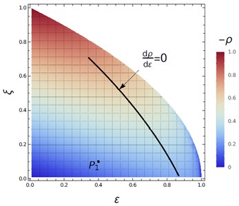
The plot provides the stability chart in the parameter space for which avoiding complex values. The white region represents the values for which the period is complex, while the region in color represents those real values for which the trivial solution of the system is exponentially stable.
The gain of the controller is determined using the stability chart by considering the estimated value of the equivalent damping ratio and choosing an appropriated value for the tuning parameter . For instance, consider the estimated damping ratio and the value . In Fig. 4 the corresponding point label as .
A greater distance from the poles to the imaginary axis allows a faster convergence to zero of the system response. For this reason, it is important to find parameter setting that maximizes this distance. Regarding the optimal , it is possible to state an optimization problem considering the root loci of the poles of the reduced linear system described in Eq. (18), that is, an appropriate stability margin can be provided by maximizing the distance between the poles and the imaginary axis.
The maximum distance is accomplished when the derivative of the pole is equal to zero, that is when . Notice that such derivative exits and corresponds to a Frechet derivative because the Floquet exponent is semi-simple [25].
Therefore, for a damping ratio , the derivative yields a transcendental equation which is solved for the optimal value applying the Newton-Rapson method. The result of this iterative procedure is shown in the contour plot by the set of points denoted by . Therefore, the set of points are the values where the distance between the poles and the imaginary axis is maximized.
On the other hand, the tuning procedure employs the stability chart to choose the tuning parameter for a given damping ratio . As expected, this design procedure entails some source of uncertainty, mainly in the identification process of the damping ratio. Therefore, it is natural to ask what about the uncertainty of the parameters; hence, we shall perform a sensitivity analysis to study the effects of parameter variations on the Floquet exponent.
3.4. Sensitivity analysis
Let consider that and are the nominal values, then the nominal Floquet exponent is given by , we wish to measure the change of as the parameters and change from their nominal values. For that aim, let denotes a change in , where represents percent changes, for example, 1, 5, 10 %, etc. For a change in the Floquet exponent yields , then, measure the variation with respect to and let denotes the percent change.
Consider , where is known as the sensitivity function of with respect to , see [26]. Then, and the relation yields:
Eq. (19) measures the change in as varies. However, the parameter may also vary then:
where . The above expression measures the change in as varies. In addition, can also vary when both parameters and have variations then:
Notice that the sensitivity functions and are well-defined since the Floquet exponent is semi-simple, and hence their respective derivative corresponds to a Frechet derivative [25].
When the tuning parameter corresponds to the optimal value the sensitivity function is approximately equal to zero since . Then, we can deduce that the controller is robust against small changes in the parameters.
4. Numerical and experimental results
In this section, we carry out the simulation and experimental verification of the switched stiffness active controller. The numerical simulation of the mass-spring system is based on the system parameters of the experimental model depicted in Fig. 5.
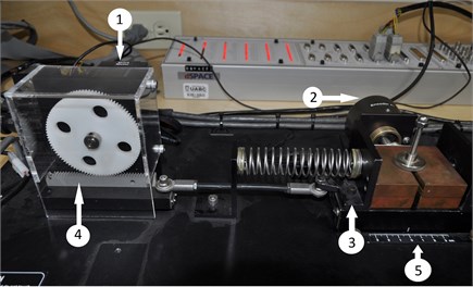
Fig. 5Mass-spring car system: 1 – actuator, 2 – optical encoder, 3 – mass-spring car, 4 – rack-and-pinion gear-set, 5 – scale of ±3.0 cm
4.1. Numerical results
The dynamics of the experimental mass-spring system can be described by Eq. (1), whose parameters correspond to: kg, N/m and Ns/m respectively, where the estimated damping ratio is equal to . The methodology to estimate the damping ratio is shown in a later section. Based on these parameter we carry out the simulation of controller.
4.1.1. Simulation
The controller gain is and the tuning parameter is chosen arbitrarily as example as in the stability chart of Fig. 4. As illustrative example, the point in the stability chart is selected, thus, the controller gain is .
The numerical solution of the controlled system Eq. (1) for the initial condition cm is plotted in Fig. 6, along with the control law Eq. (2) and the switching function.
The mass-spring system under the action of the controller becomes a linear periodic system, whose multiplier and Floquet exponent are calculated by Eq. (16-17), that is, and respectively. To validate our predictions, the Floquet exponent may roughly be estimated from the numerical solution using the logarithmic decrement technique. From Fig. 6(a) the logarithmic decrement approximates the Floquet exponent. The error in the approximation is because the actual system response can not the approximated by the oscillatory response of the second-order linear system as the logarithmic decrement technique intends to do.
Notice the amount of stiffness introduced into the system is given by relation . On the other hand, the design procedure of the controller entails some sources of uncertainty, due mainly to the damping ratio identification. To overcome this disadvantage and to show the robustness of the controller against parameter uncertainty, a sensitivity analysis is carried out in the following.
4.1.2. Robustness analysis
The nominal parameters are and the corresponding Floquet exponent is . We consider that both parameters vary, then Eq. (19) is used to tabulate, in Table 1, the sensitivity analysis results. The table relates the percent variations of the Floquet exponent due to variations of the parameters .
Fig. 6Numerical solution of the control system Eq. (1) where m=1.2 kg, b=4.5 N/m, k=487.8 Ns/m and kc=195: a) position x^p, b) corresponding control law u, c) switching function
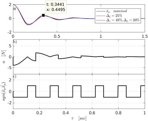
The data in Table 1 is interpreted as follows. For instance, consider a variation of 25 % of the parameter with no variations in , then from the table 1 the percent variation is 14 %. As second example, now consider a variation in both nominal parameters, for instance, with 20 % and with 10 %, then Floquet exponent has a variation of . In both examples, the corresponding results are pointed out in table 1 by the color text.
Table 1Percent variation Δρ/ρ0 of the Floquet exponent ρ0=0.215485 as parameters vary from their nominal values (ξ0,ε0)=(0.0932,0.4)
, % | , % | ||||
0 | 5 | 10 | 25 | 30 | |
0 | 0 | 3 | 6 | 14 | 17 |
10 | 5 | 8 | 11 | 19 | 22 |
20 | 9 | 12 | 15 | 23 | 26 |
30 | 13 | 16 | 19 | 27 | 30 |
50 | 21 | 24 | 27 | 35 | 38 |
To visualize the effect of parameters variation on the system response, two examples are plotted in Fig. 6(a). The corresponding solutions of Eq. (1) that shows with no variation in (bolded) and a variation in both parameters as , (blue).
In addition, the Euclidean norm of the solution may be used as a quantitative measure for validate the robustness of the controller, i.e., for the nominal solution , and for the present examples and respectively. From the above sensitivity analysis, one deduces that the controller is robust against parameter uncertainty.
4.2. Experimental model
The experimental model is comprised of the mass-spring car which is constrained to move horizontally on a rail, an optical encoder which measures mass motion, a DC servomotor with a rack-and-pinion gear-set adaptation which provides the control action; notice that the distance traveled by the mass is ±3 cm. Besides, Fig. 7 shows the fully assembled experimental setup. The dSPACE data acquisition platform is used to register the experimental data and to implement the control law in real-time by using the block diagram formulation through the Matlab/Simulink software, where the sample time of the data acquisition is ms.
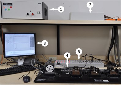
Fig. 7Experimental rig: 1 – power supply, 2 – dSPACE computer, 3 – PC with Matlab/Simulink, 4 – ECP rectilinear plant model 201, 5 – dSPACE panel connector
The mass-spring car experiments a friction force during its motion. For practical purposes, we assume that such force can be quantified by a linear viscous damping force, where the logarithmic decrement technique is applied to estimate the damping coefficient.
To apply the technique, the free vibration response is experimentally determined considering the initial position cm. and zero initial velocity. The period of the free vibration response is found as seg. and a second peak amplitude . From the logarithmic decrement we have , then, solving for the damping ratio yields .
The stiffness and damping parameters are calculated by the relations , and , where the mass is equal to Kg. Thus, the parameters are approximately equal to N/m and Ns/m respectively.
4.3. Experimental verification
A crucial step in the controller implementation is to calculate the switching function since the velocity must be obtained. Therefore, the controller performance is based on which technique is used to calculate the velocity. One common technique is the numerical differentiation of the position, but this approach may yield a velocity contaminated by noise. A second approach is the use of state observers, but this approach depends on an appropriate choose of the observer and the tuning of its gains. Nevertheless, in this paper, we developed a novel and heuristic approach to calculate the switching function without velocity measurement, where we take into account the dynamics of the mass during its motion.
4.3.1. Switching function calculation
To explain how we calculate the switching function without velocity measurement, we compare our approach to the position differentiation approximation scheme. The state observer formulation is not considered in the following comparison.
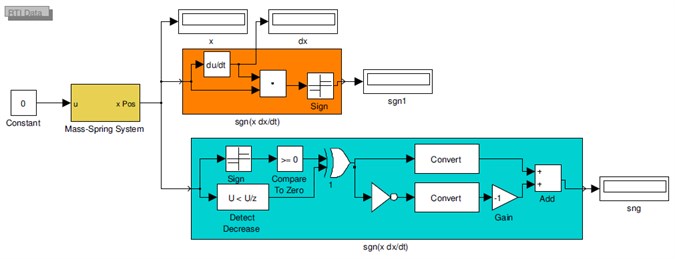
Fig. 8 shows the Matlab/Simulink block diagram for the experimental implementation of both approaches. The orange block calculates the switching function by differentiating the position while the cyan block executes the algorithm to calculate the switching function without the velocity measurement. The yellow block explained in the appendix corresponds to the input-output data acquisition relations of the experiment setup. The block diagram is converted to computer code and loaded into the dSPACE real-time platform which runs at a sample time of ms.
Fig. 8Block diagram for calculating the switching function sgn(xx˙) without measure the velocity
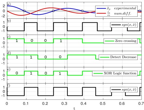
The experiment results of both approaches are shown in Fig. 9. Where Fig. 9(a) shows the position of the mass and its velocity, which has been calculated by numerical differentiation, for illustrative purposes, the velocity is scaled by the natural frequency, that is, . The corresponding switching function based on numerical differentiation is plotted in Fig. 9(b).
Even when, in this particular case, the numerical differentiation scheme provides quite good agreement with our approach, it is well-known that it may be susceptible to be contaminated by noise and; and, in general, it is avoided.
We base our approach on the motion of the mass. The approach determines when the position crosses the zero and when it is decreasing, these operations yield the two logic signals plotted in Fig. 9(c) and Fig. 9(d) respectively. The exclusive OR logic operation between these signals yields the signal plotted in Fig. 9(e), and finally the signal conditioning yields the switching function plotted in Fig. 9(f) this signal is the same of Fig. 9(b). Therefore, our approach does not require velocity measurement, in this way the control law is implemented.
Fig. 9Time history of the signals used for calculating the switching function
4.3.2. Experimental results
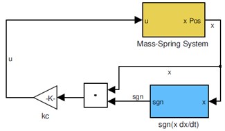
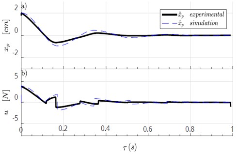
Fig. 10 shows the block diagram to implement the controller, the blue block calculate the switching function. The experimental results of the control law 2 are shown in Fig. 11, for control gain used in the numerical simulation. For comparative purposes, in Fig. 11 we plot the experimental response and the numerical simulation .
Fig. 10Block diagram of the controller implementation for the mass-spring system
Notice that there is a discrepancy between the experimental result and the solution. This fact is due mainly to the action of additional dynamics not taken into account in the model like the dry friction, the backlash of the rack-and-pinion gear-set, and the induced dynamic by the DC servomotor. Nevertheless, the controller is robust and can handle these drawbacks.
Fig. 11Experimental result of the control system with kc=195
5. Conclusions
The switched stiffness technique is a semi-active vibration control technique achieved by semi-active stiffness devices to change the total system stiffness to mitigate the vibration in structures. The system response depends on the parameters of the involved semi-active device, however, in real-world situations, the semi-active device cannot handle the optimal values that improve the system response. Consequently, the limitations of the switched stiffness technique are increasingly apparent.
To tackle this issue, the authors developed a feasible controller to vibration mitigation of a single-degree-of-freedom system where the dissipative phenomenon is considered. We show that the vibration control system behaves periodically in time, this remarkable fact allows us to analyze the system as a periodic differential equation, where the Floquet theory is applied to establish closed analytic expression for stability conditions in terms of parameters system instead of linear approximations. This allows us to prove the exponential stability of the system, to provide a tuning scheme for the controller gain, to perform an optimization process and to show the robustness of the controller by carrying out a sensitivity analysis.
Besides, the conducted experimental verification shows good agreement with the theoretical analysis and supports and validates our approach. The controller can be extended to be used for shock isolation.
References
-
Chen J. C. Response of large space structures with stiffness control. Journal of Spacecraft and Rockets, Vol. 21, Issue 5, 1984, p. 463-467.
-
Onoda J., Endot T., Tamaoki H., Watanabe N. Vibration suppression by variable-stiffness members. AIAA Journal, Vol. 29, Issue 6, 1991, p. 977-983.
-
Onoda J., Sanot T., Kamiyama K. Active, passive, and semiactive vibration suppression by stiffness variation. AIAA Journal, Vol. 30, Issue 12, 1992, p. 2922-2929.
-
Goh C. J., Caughey T. K. A quasi-linear vibration suppression technique for large space structures via stiffness modification. International Journal of Control, Vol. 41, Issue 3, 1985, p. 803-812.
-
Ramaratnam A., Jalili N. A switched stiffness approach for structural vibration control: Theory and real-time implementation. Journal of Sound and Vibration, Vol. 291, Issues 1-2, 2006, p. 258-274.
-
Leavitt J., Jabbar F., Bobrow J. E. Optimal performance of variable stiffness devices for structural control. Journal of Dynamic Systems, Measurement and Control, Transactions of the ASME, Vol. 129, Issue 2, 2007, p. 171-177.
-
Ledezma Ramirez D., Ferguson N., Brennan M. An experimental switchable stiffness device for shock isolation. Journal of Sound and Vibration, Vol. 331, Issue 23, 2012, p. 4987-5001.
-
Scheidler J. J., Asnani V. M., Dapino M. J. Dynamically tuned magnetostrictive spring with electrically controlled stiffness. Smart Materials and Structures, Vol. 25, Issue 3, 2016, p. 035007.
-
Winthrop M. F., Baker W. P., Cobb R. G. A variable stiffness device selection and design tool for lightly damped structures. Journal of Sound and Vibration, Vol. 287, Issues 4-5, 2005, p. 667-682.
-
Adhikari S., Woodhouse J. Identification of damping. Part I: Viscous damping. Journal of Sound and Vibration, Vol. 251, Issue 3, 2002, p. 477-490.
-
Liang J. W., Feeny B. F. Identifying coulomb and viscous friction from free-vibration decrements. Nonlinear Dynamics, Vol. 16, Issue 4, 1998, p. 337-347.
-
Reid T. J. Free vibration and hysteretic damping. The Journal of the Royal Aeronautical Society, Vol. 60, 1956, p. 544-283.
-
Bert C. Material damping. Journal of Sound and Vibration, Vol. 29, Issue 2, 1973, p. 129-153.
-
Caughey T. K., Vijayaraghavan A. Free and forced oscillations of a dynamic system with “linear hysteretic damping” (non-linear theory). International Journal of Non-Linear Mechanics, Vol. 5, Issue 3, 1970, p. 533-555.
-
Zhang Y., Iwan W. D. Some observations on two piecewise-linear dynamic systems with induced hysteretic damping. International Journal of Non-Linear Mechanics, Vol. 38, Issue 5, 2003, p. 753-765.
-
Caughey T., Vijayaraghavan A. Stability analysis of the periodic solution of a piecewise-linear non-linear dynamic system. International Journal of Non-Linear Mechanics, Vol. 11, Issue 2, 1976, p. 127-134.
-
Caughey T., Vijayaraghavan A. Forced oscillations of a piecewise-linear non-linear dynamic system with several degrees of freedom. International Journal of Non-Linear Mechanics, Vol. 12, Issue 6, 1977, p. 339-353.
-
Inaudi J. A. Modulated homogeneous friction: a semi–active damping strategy. Earthquake Engineering and Structural Dynamics, Vol. 26, Issue 3, 1997, p. 361-376.
-
Liu C. S. Reid’s passive and semi-active hysteretic oscillators with friction force dependence on displacement. International Journal of Non-Linear Mechanics, Vol. 41, Issues 6-7, 2006, p. 775-786.
-
Moreno Ahedo L., Diarte Acosta S. Stability analysis of linear systems with switchable stiffness using the Floquet theory. Journal of Vibration and Control, Vol. 25, Issue 5, 2019, p. 963-976.
-
Khalil H. K. Nonlinear Systems. Prentice Hall, New York, 2nd edition, 1996.
-
Garrido H., Curadelli O., Ambrosini D. On the assumed inherent stability of semi-active control systems. Engineering Structures, Vol. 159, 2018, p. 286-298.
-
Liang J. W. Damping estimation via energy-dissipation method. Journal of Sound and Vibration, Vol. 307, Issue 1, 2007, p. 349-364.
-
Calogero F. Isochronous Systems. Oxford University Press, Oxford, 2008.
-
Sun J. G. Sensitivity analysis of multiple eigenvalues (I). Journal of Computational Mathematics, Vol. 1, Issue 1, 1988, p. 28-38.
-
Frank P. M. Introduction to System Sensitivity Theory. Academic Press, New York, 1978.
-
Yakubovich V. A., Starzhinskii V. M. Linear Differential Equations with Periodic Coefficients. Wiley, New York, 1975.
-
Montagnier P., Paige C. C., Spiteri R. J. Real Floquet factors of linear time-periodic systems. Systems and Control Letters, Vol. 50, Issue 4, 2003, p. 251-262.
About this article

