Abstract
Variational mode decomposition (VMD) is a recently introduced adaptive signal decomposition algorithm with a solid theoretical foundation and good noise robustness compared with empirical mode decomposition (EMD). There is a lot of background noise in the vibration signal of diesel engine. To solve the problem, a denoising algorithm based on VMD and Euclidean Distance is proposed. Firstly, a multi-component, non-Gauss, and noisy simulation signal is established, and decomposed into a given number K of band-limited intrinsic mode functions by VMD. Then the Euclidean distance between the probability density function of each mode and that of the simulation signal are calculated. The signal is reconstructed using the relevant modes, which are selected on the basis of noticeable similarities between the probability density function of the simulation signal and that of each mode. Finally, the vibration signals of diesel engine connecting rod bearing faults are analyzed by the proposed method. The results show that compared with other denoising algorithms, the proposed method has better denoising effect, and the fault characteristics of vibration signals of diesel engine connecting rod bearings can be effectively enhanced.
Highlights
- A new method based on VMD and Euclidean distance is proposed.
- The denoising method proposed in this paper is effective for the vibration signals of diesel engine.
- Compared with EMD-ED and VMD-CORR, the denoising method proposed is more effective.
1. Introduction
Vibration signal processing has been an effective way of monitoring mechanical equipment for many years. However, mechanical vibration signal are usually masked by significant background noise, which have motivated many studies into developing denoising methods [1]. The vibration signals should be processed to reduce noise and improve the quality before further analyzing [2]. Many researchers in this field have made thorough explorations. Wavelet denoising is a very effective denoising method in recent years, among which wavelet threshold denoising is the most commonly used method [3-6]. However, the denoising effect of this method is affected by the selection of basis functions and depends on the subjective experience of the designer, which has uncertainty.
In order to solve the above problems, Huang et al. introduced an adaptive signal processing technique called empirical mode decomposition (EMD) [7, 8], which has demonstrated outstanding performance in dealing with nonlinear and nonstationary signals. This technique has been applied in many fields, such as biomedical image analysis [9], fault diagnosis of rolling element bearings [10], signal de-noising [11-13], and voice signal analysis [14]. According to the principle of wavelet threshold denoising, EMD threshold denoising is put forward [15, 16].
Euclidean distance, as an old method, is widely used to judge the similarity between vectors and image recognition and so on. Many researchers have studied the Euclidean distance in depth. Wang [17] et al. used Euclidean distance for image recognition. Wu [18] et al. used Euclidean distance to identify objects and scenes. Santhanam [19] et al. used Euclidean distance for image denoising. In addition, EMD denoising combined with the Euclidean distance (ED) is proposed in document [20]. All these methods have achieved good denoising effect. However, EMD still has some disadvantages, such as mode mixing and the lack of an exact mathematical model of the process.
In recent years, Konstantin Dragomiretskiy et al. proposed variational modal decomposition [18], which is essentially composed of several adaptive Wiener filters and has good noise robustness. Compared with EMD, VMD has strong mathematical theory basis. So, it can effectively alleviate or avoid a series of problems that exist in EMD, and has higher operation efficiency. VMD is widely used in various engineering fields [21-25]. An X. L. et al. applied VMD to the bearing fault diagnosis of the wind turbine, and realized the effective discrimination of the bearing fault [26]. By combining VMD with detrended fluctuation analysis (DFA), Liu et al. successfully extracted gear fault characteristics [27]. By combining VMD with independent component analysis (ICA), Yao et al. successfully separated the piston knock and combustion noise of the engine [28]. Zhang M. et al. proposed a denoising method based on VMD and correlation coefficient (VMD-CORR) [29]. However, because of the large amount of noise in the signal, it is easy to remove the useful components in the signal, which leads to the distortion of the signal.
In this paper, a denoising algorithm, called the VMD-Euclidean distance (VMD-ED), is presented for vibration signal of diesel engine. Firstly, a multi-component, non-stationary and non-Gauss simulation signal is established, and the Gauss white noise is added. Secondly, the simulation signal is decomposed by VMD to obtain the band limited intrinsic mode functions (BLIMFs). Then the probability density functions (PDF) of the simulation signal and each BLIMF are calculated respectively, and the ED between the PDF of the simulation signal and that of each BLIMF is calculated. A smaller ED value means that more features are contained in the signal under comparison; the relevant modes are thus selected to reconstruct the signal. To validate the denoising effect of the proposed scheme, several denoising methods are compared with VMD-ED under different evaluation criteria, including the root mean square error (RMSE), mean absolute error (MAE), and the output signal-to-noise ratio (SNR out). Compared with the denoising methods of document [20, 29], the method proposed in this paper has better denoising effect. Finally, the noise of the fault signals of diesel engine connecting rod bearings is effectively eliminated by using VMD-ED, and the fault characteristic is highlighted.
2. Variational mode decomposition
The VMD algorithm defines the intrinsic mode function as a non-stationary AM-FM signal. The intrinsic mode is considered as follows:
where the phase shall satisfy the following condition: 0; the envelope line should satisfy the following condition: 0; the instantaneous frequency should satisfy the following condition:. and change slowly, and changes more rapidly.
The Hilbert transform is performed for each modal function , and exponential correction is applied to obtain modal functions. Then the frequency spectrum of the modal function is corrected to the estimated central frequency, and the bandwidth of the modal component is calculated by using Gauss smoothing. The variational constraint problem can be defined as follows:
where is the modal component, is the central frequency for the modal component, is the unit pulse function, and * is the convolution symbol.
In the VMD algorithm, the secondary penalty factor and the Lagrangian multiplication operator are used. Then, the alternating direction method is introduced. , , and are constantly updated, so that the optimal solution of the variational constraint problem can be solved. The expression for the modal component is:
where is the penalty factor, and is the Lagrange multiplier.
The expression for the modal component in frequency domain is:
where is the center of the modal component power spectrum. The Wiener filter is introduced, which makes the VMD algorithm have better noise robustness.
Similarly, the expression for the central frequency is:
The stopping condition of the iteration is:
The VMD algorithm is a linear transformation, so the signal can be reconstructed. The reconstructed signal can be represented as:
where is the final modal component, after the iteration is stopped.
3. Euclidean distance
The vibration signals of vehicle structures are mostly symmetrical non-Gauss signals. The PDF is calculated according to the Gauss curve stitching method based on empirical information, which is proposed by Steinwolf [30]. The PDF can fully reflect the statistical characteristics, the distribution law, the cumulant and the statistical moments of each order for non-Gauss signals. By comparing the ED between the PDF of the simulation signal and that of each BLIMF, the real BLIMFs can be selected to reconstruct the signal.
The PDF of the signal can be regarded as a point in the dimensional space, and the ED between the point A and the point B can be represented as:
where the coordinates of the point A are (, , …, ), and the coordinates of the point B are (, , …, ). The ED reflects the similarity of the two signals as the basis for signal reconstruction.
4. Proposed method
Vibration signal analysis is usually used for condition monitoring and fault diagnosis. However, due to the complex structure of diesel engines, the vibration signals of diesel engines are usually multi-component, non-stationary and non-Gauss. In addition, there is a large amount of background noise in the vibration signals of diesel engines. Therefore, it is very difficult to extract fault characteristics from the vibration signals of diesel engines.
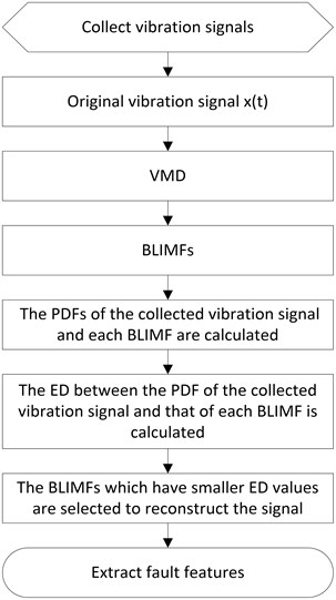
VMD is a recently proposed signal decomposition method, which is essentially composed of a number of adaptive Wiener filters and has good noise robustness. Compared with the EMD method, the VMD method has a solid mathematical theoretical foundation, and can effectively alleviate or avoid a series of shortcomings in the EMD method. To verify the efficiency of the proposed method, several experiments on diesel engine connecting rod bearings faults are performed. The detailed experimental scheme is shown in Fig. 1. Firstly, a signal channel vibration , which is a wearing fault of the diesel engine connecting rod, is collected by the acceleration sensor vertically fixed on the diesel engine block. Secondly, the collected vibration signal is decomposed into six BLIMFs by VMD method. Thirdly, the PDFs of the collected vibration signal and each BLIMF are calculated respectively, and the ED between the PDF of the collected vibration signal and that of each BLIMF is calculated. Lastly, the relevant modes, which have smaller ED values, are thus selected to reconstruct the signal.
Fig. 1Detailed experimental scheme. BLIMF, band limited intrinsic mode functions; PDFs, probability density functions; ED, Euclidean distance
5. Experimental results
5.1. Simulation
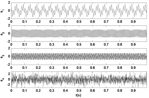
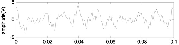
Because of the complex structure of diesel engine, the number of vibration excitation source is large, and the vibration source signal is modulated by several components. Therefore, the established simulation signal must be multi-component and non-Gauss. According to document [31], the simulation signals are performed to verify the effectiveness of the proposed method, expressed in Eq. (13)-(18). The mixed signal consists of three components, and the fault characteristic frequencies of the mixed signal are 50, 150 and 250 Hz. In addition, the mixed signal consists of four components, and the fourth component is the Gauss white noise:
where is the original simulation signal before adding noise, and is the noisy simulation signal after adding noise. The waveforms of the four components are shown in Fig. 2.
Fig. 2Source simulation signals
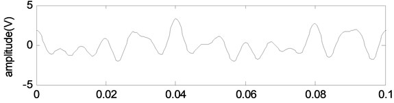
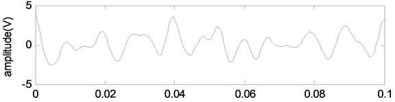
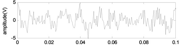
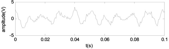
The sampling frequency is 2048 Hz, and the number of sampling points is 2048. The two mixed signals in the time domains are shown in Fig. 3. As we can see from Fig. 3, the shock component in the signal is weakened and the simulation signal becomes very cluttered, which is not convenient for fault feature extraction.
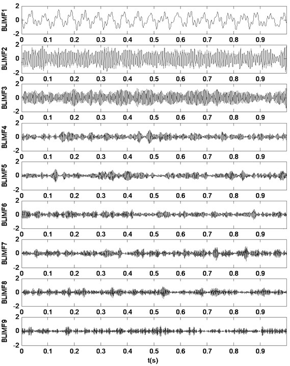
Then, according to the detailed experimental scheme shown in Fig. 1, the mixed signal is first decomposed into nine BLIMFs by the VMD method. The nine BLIMFs are shown in Fig. 4.
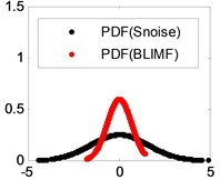
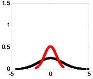
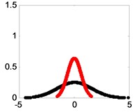
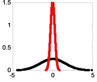
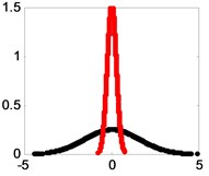
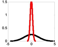
As we can see from Fig. 4, pseudo component appears in the nine BLIMFs. Then the PDFs of the mixed signal and each BLIMF are calculated respectively. The PDFs are shown in Fig. 5.
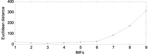
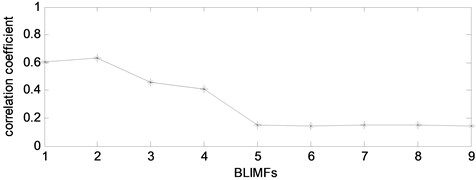
As we can see from Fig. 5, the PDFs of different BLIMF are not the same. In order to compare the differences among the BLIMFs more accurately, the Euclidean distance between the PDF of each BLIMF and that of the mixed signal is calculated respectively. Similarly, the Euclidean distance between the PDF of each IMF and that of the mixed signal is calculated by the EMD-ED method, and the correlation coefficient between each BLIMF and the mixed signal is calculated by the VMD-CORR method, as shown in Fig. 6 and Table 1.
Fig. 3Simulation signals: a) waveform of the mixed signal Soriginal, b) waveform of the mixed signal Snoise
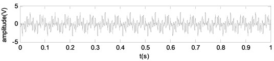
a)

b)
Fig. 4BLIMFs decomposed by the VMD method
As can be seen from Fig. 6 and Table 1, for the proposed method, the Euclidean distance of the first 3 BLIMFs is obviously smaller than that of other BLIMFs, which is consistent with the composition of the mixed signals. According to the experimental analysis, the Euclidean distance threshold is set to 20, and the BLIMFs with Euclidean distance less than 20 are used as the component of the reconstructed signal. Therefore, the first 3 BLIMFs are selected to reconstruct the signal to obtain the denoised signal. Similarly, using the EMD-ED and VMD-CORR methods mentioned above, the denoised signal is obtained. A part of the reconstructed signal is selected, and the reconstructed signals obtained by different methods are shown in Fig. 7.
Fig. 5Superposition of the PDF of Snoise and those of its BLIMFs
a) BLIMF 1
b) BLIMF 2
c) BLIMF 3
d) BLIMF 4

e) BLIMF 5
f) BLIMF 6

g) BLIMF 7

h) BLIMF 8
i) BLIMF 9
Table 1Comparison of different methods
VMD | Euclidean distance | EMD | Euclidean distance | VMD | Correlation coefficient |
BLIMF1 | 11.63 | IMF1 | 24.65 | BLIMF1 | 0.60 |
BLIMF2 | 8.62 | IMF2 | 12.19 | BLIMF2 | 0.63 |
BLIMF3 | 13.68 | IMF3 | 10.47 | BLIMF3 | 0.45 |
BLIMF4 | 92.37 | IMF4 | 16.15 | BLIMF4 | 0.41 |
BLIMF5 | 108.7 | IMF5 | 22.12 | BLIMF5 | 0.15 |
BLIMF6 | 111.4 | IMF6 | 25.87 | BLIMF6 | 0.14 |
BLIMF7 | 102.6 | IMF7 | 86.37 | BLIMF7 | 0.15 |
BLIMF8 | 97.58 | IMF8 | 173.2 | BLIMF8 | 0.15 |
BLIMF9 | 97.81 | IMF9 | 313.4 | BLIMF9 | 0.14 |
As we can see from Fig. 7, the reconstructed signal obtained by the proposed method is more similar to the mixed signal . The noise in the signal is effectively removed, and the shock component is highlighted. Therefore, the method proposed in this paper is more effective in denoising. In the reconstructed signals obtained by EMD-ED, VMD-CORR and wavelet, there are many spikes, which are very different from the original signal. Thus, the denoising effect of the three methods is not as good as the proposed method.
In order to evaluate the performance of different methods more comprehensively, different intensities of noise signals (–10-30 dB) are added to the simulation signals. The signal to noise ratio (SNR), the root mean square error (RMSE) and the mean absolute error (MAE) of the reconstructed signals obtained by different methods are calculated respectively, as shown in Fig. 8.
As we can see from Fig. 8, the SNR of the proposed method is significantly higher than that of the other three methods, and RMSE and MAE are significantly lower than those of the other three methods. Therefore, the method proposed in this paper is better than other three methods in denoising.
Fig. 6Comparison of different methods
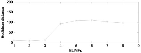
a) VMD-ED
b) EMD-ED
c) VMD-CORR
5.2. Experiment condition
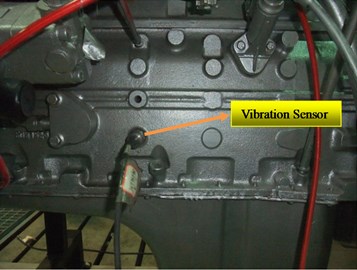
The structure of diesel engine is complex and the working environment is abominable. As a result, it is prone to malfunction. The connecting rod bearing is located inside the engine, so it is difficult to diagnose the fault. In this paper, vibration signals are collected from the vibration sensors on the experimental stand, as shown in Fig. 9. The basic parameters of the vibration sensor are shown in Table 2. The engine on the experimental stand is Cummins 6BT diesel engine, and its parameters are shown in Table 3.
Table 2Vibration sensor parameters
Model | Sensitivity | Frequency range (±3 dB) | Range | Resolution | Temperature range | Weight | Output connector |
603C01 | 100 mV/g | 0.5 Hz-10 KHz | ±50 g | 350 μg | –54-121℃ | 51 g | Top |
Table 3Basic parameters of the engine
Engine type | 6BT5.9-G2 | Fuel type | Diesel oil | Type | Inline 6 cylinders |
Rated power (KW) | 118 | Compression ratio | 17.5:1 | Ignition sequence | 153624 |
Rated speed (RPM) | 2600 | Continuous power (KW) | 86 | Maximum torque (N·m) | 558 |
Radius (mm) × Distance (mm) | 102×120 | Maximum torque Speed (r/min) | 1600 | ||
The fourth connecting rod bearings of Cummins EQ6BT diesel engine are set with different clearance (0.10 mm, 0.14 mm, 0.20 mm, 0.34 mm) to simulate the normal, minor, moderate and severe wear of the connecting rod bearing. Vibration signals are collected on the left side of the fourth main bearings on the surface of the engine block. The sampling frequency is 20000 Hz and the sampling points are 4096 points.
Testing temperature is important when acquiring vibration signals. In the experiment, the temperature of cooling water is measured to reflect the internal temperature of diesel engine. The temperature is controlled at 60-70 °C.
Fig. 7The reconstructed signals obtained by different methods
a) Original signal
b) VMD-ED
c) VMD-CORR
d) EMD-ED
e) Wavelet
5.3. Data acquired
The acquisition system is composed of collector, computer, sensor and connecting circuit, as shown in Fig. 10. According to document [4], the optimum diagnostic speed of this type of diesel engine is 1800 r/min. In addition, four speeds were collected in the experiment: 800 r/min, 1300 r/min, 1800 r/min, and 2100 r/min. The experiment proved that 1800 r/min is the most suitable for the fault diagnosis speed. Therefore, the acquisition system set the speed of the engine to 1800 r/min.
Fig. 8Comparison of denoising effects of different methods
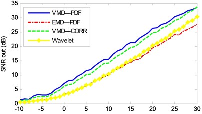
a) SNR
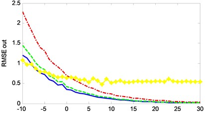
b) RMSE
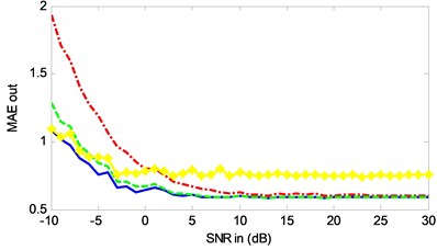
c) MAE
Fig. 9Measuring position of vibration sensor
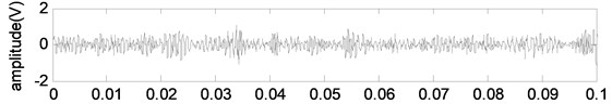
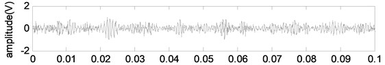
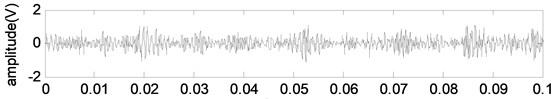
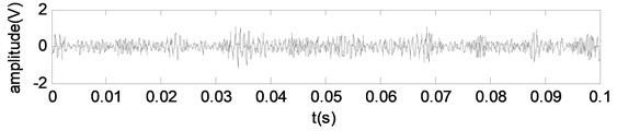
The vibration signals of the engine under different wear conditions are collected, as shown in Fig. 11. In Fig. 11, there is a large amount of background noise in the vibration signals of different wear conditions of the connecting rod, which is unfavorable to the extraction of fault features. The signal energy values of different wear conditions are then calculated, as shown in Table 4.
Fig. 10Vibration signal acquisition system
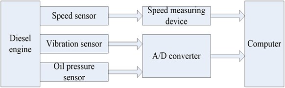
Fig. 11Vibration signals of connecting rod bearing under different wearing conditions
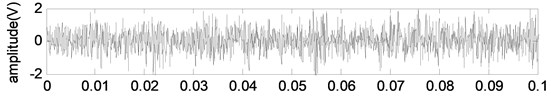
a) Normal wear
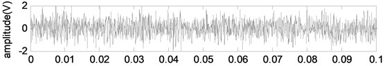
b) Minor wear
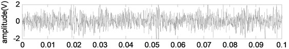
c) Moderate wear

d) Severe wear
From Table 4, it can be seen that there is no regularity in the signal energy of different wear conditions. Therefore, the fault features of the signal can not be extracted, and the signal needs to be further processed.
Table 4The signal energy of different wear conditions before the signal de-noising
Wear condition | Normal wear | Minor wear | Moderate wear | Severe wear |
Signal energy | 1027.9 | 989.3 | 999.2 | 940.6 |
5.4. Experimental data processing
The vibration signal of connecting rod bearing is analyzed according to the method proposed in this paper. The Euclidean distance between the PDF of each BLIMF and that of the vibration signals under different wear conditions is shown in Fig. 12 and Table 5.
Fig. 12The Euclidean distance between the PDF of each BLIMF and that of the vibration signals under different wear conditions
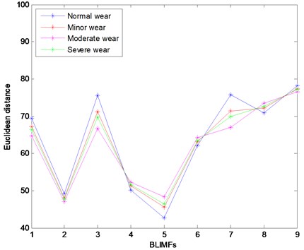
Table 5The Euclidean distance between the PDF of each BLIMF and that of the vibration signals under different wear conditions
BLIMFs | Normal wear | Minor wear | Moderate wear | Severe wear |
BLIMF1 | 69.39 | 67.08 | 64.78 | 66.31 |
BLIMF2 | 49.16 | 48.08 | 47.00 | 47.72 |
BLIMF3 | 75.64 | 71.18 | 66.73 | 69.70 |
BLIMF4 | 50.12 | 51.21 | 52.30 | 51.58 |
BLIMF5 | 42.62 | 45.51 | 48.40 | 46.47 |
BLIMF6 | 62.06 | 63.13 | 64.20 | 63.48 |
BLIMF7 | 75.74 | 71.40 | 67.05 | 69.95 |
BLIMF8 | 70.82 | 72.17 | 73.52 | 72.62 |
BLIMF9 | 78.23 | 77.42 | 76.60 | 77.15 |
As we can see from Fig. 12 and Table 5, the Euclidean distance of the BLIMF2, BLIMF4 and BLIMF5 is obviously smaller than that of other BLIMFs for the vibration signals under different wear conditions. According to the experimental analysis, the Euclidean distance threshold is set to 60, and the BLIMFs with Euclidean distance less than 60 are used as the component of the reconstructed signal. Therefore, the BLIMF1, BLIMF4 and BLIMF5 are selected to reconstruct the signal. A part of the reconstructed signal is selected, and the reconstructed signals under different wear conditions are shown in Fig. 13.
Fig. 13The reconstructed signals under different wear conditions
a) Normal wear
b) Minor wear
c) Moderate wear
d) Severe wear
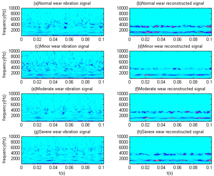
As we can see from Fig. 13, in the reconstructed signals under different wear conditions, the noise is reduced effectively. As compared with Fig. 11, the signals become smoother and the shock components are more obvious. In order to further investigate the denoising effect of the proposed method, the vibration signals and reconstructed signals of different wear conditions are transformed by Morlet wavelet, as shown in Fig. 14. The signal energy values of different wear conditions are then calculated, as shown in Table 6.
Table 6The signal energy of different wear conditions after the signal de-noising
Wear condition | Normal wear | Minor wear | Moderate wear | Severe wear |
Signal energy | 389.0 | 413.2 | 446.1 | 476.2 |
As we can see from Fig. 14, compared with the vibration signals, the noise is effectively suppressed in the reconstructed signals, and the fault characteristics are obviously enhanced. From Table 6, we can see that with the deterioration of the wear condition, the signal energy value increases gradually. Thus, the denoising method proposed in this paper is effective.
Fig. 14Time frequency analysis of vibration signals and reconstructed signals under different wear conditions
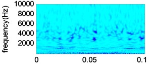
a) Normal wear vibration signal
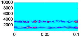
b) Normal wear reconstructed signal
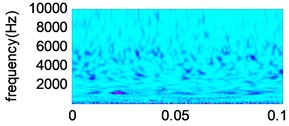
c) Minor wear vibration signal
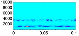
d) Minor wear reconstructed signal
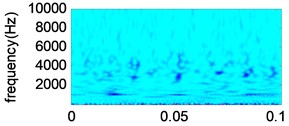
e) Moderate wear vibration signal
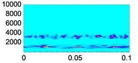
f) Moderate wear reconstructed signal
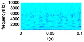
g) Severe wear vibration signal
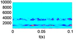
h) Severe wear reconstructed signal
6. Conclusions
A new method based on VMD and Euclidean distance is proposed for diesel engine vibration signals, which usually contain a large amount of background noise. Firstly, the vibration signals are decomposed into several BLIMFs. Secondly, the PDFs of the vibration signals and each BLIMF are calculated respectively, and the Euclidean distance between the PDF of each BLIMF and that of the vibration signals is calculated. Finally, the BLIMFs with smaller Euclidean distance value are selected to reconstruct the signal. Compared with EMD-ED and VMD-CORR, the denoising method proposed in this paper is more effective. The proposed method is applied to the vibration signals of diesel engine connecting rod bearing wear faults. The noise is effectively suppressed, and the fault characteristics are obviously enhanced. However, the proposed method needs a given number of BLIMFs when vibration signal is decomposed by VMD, which is a drawback currently. Future work will focus on further optimization of the proposed method.
References
-
Chen Y., Zhang P., Wang Z., Yang W., Yang Y. Denoising algorithm for mechanical vibration signal using quantum Hadamard transformation. Measurement, Vol. 66, 2015, p. 168-175.
-
Xie Z. J., Song B. Y., Zhang Y., Zhang F. Application of an improved wavelet threshold denoising method for vibration signal processing. Advanced Materials Research, Vol. 889, Issue 890, 2014, p. 799-806.
-
Tang J. Y., Chen W. T., Chen S. Y., Zhou W. Wavelet-based vibration signal denoising with a new adaptive thresholding function. Journal of Vibration and Shock, Vol. 28, Issue 7, 2009, p. 118-121.
-
Gao R. Study on vibration signal denoising of electric spindle based on wavelet transform. International Conference on Intelligent Human-machine Systems and Cybernetics, 2009.
-
Gao R. Analysis on singularity of fault signals of high spindle based on Hermitian wavelet. Journal of Computers, Vol. 6, Issue 4, 2011, p. 755-760.
-
To A. C., Moore J. R., Glaser S. D. Wavelet denoising techniques with applications to experimental geophysical data. Signal Processing, Vol. 89, Issue 2, 2009, p. 144-160.
-
Huang N. E., Shen Z., Long S. R. The empirical mode decomposition and the Hilbert spectrum for nonlinear and non-stationary time series analysis. Proceedings of the Royal Society A, Vol. 454, 1998, p. 903-995.
-
Huang N. E., Shen Z., Long S. R. A new view of non- linear water waves: the Hilbert spectrum. Annual Review of Fluid Mechanics, Vol. 31, 1999, p. 417-457.
-
Ai L., Wang J., Yao R. Classification of parkinsonian and essential tremor using empirical mode decomposition and support vector machine. Digital Signal Process, Vol. 21, Issue 4, 2011, p. 543-550.
-
Su W. S., Wang F. T., Zhang Z. X., et al. Application of EMD denoising and spectral kurtosis in early fault diagnosis of rolling element bearings. Journal of Vibration and Shock, Vol. 22, Issue 1, 2010, p. 3537-3540.
-
Lahmiri, Boukadoum M. A weighted bio-signal denoising approach using empirical mode decomposition. Biomedical Engineering Letters, Vol. 5, Issue 2, 2015, p. 131-139.
-
Huang C., Wang H., Long B. Signal denoising based on EMD. IEEE Circuits and Systems International Conference on Testing and Diagnosis, 2009.
-
Zhang Y. K., Ma X. C., Hua D. X., et al. An EMD-based denoising method for lidar signal. International Congress on Image and Signal Processing, Vol. 8, 2010, p. 4016-4019.
-
Khaldi K., Turki Hadj Alouane M., et al. A new EMD denoising approach dedicated to voiced speech signals. International Conference on Signals, 2008.
-
Kopsinis Y., Mclaughlin S. Development of EMD-based denoising methods inspired by wavelet thresholding. IEEE Transactions on Signal Processing, Vol. 57, Issue 4, 2009, p. 1351-1362.
-
Yang G., Liu Y., Wang Y., et al. EMD interval thresholding denoising based on similarity measure to select relevant modes. Signal Processing, Vol. 109, 2015, p. 95-109.
-
Wang L., Zhang Y., Feng J. On the Euclidean distance of images. IEEE Transactions on Pattern Analysis and Machine Intelligence, Vol. 27, Issue 8, 2005, p. 1334-1339.
-
Wu J., Rehg J. M. Beyond the Euclidean distance: creating effective visual codebooks using the histogram intersection Kernel. International Conference on Computer Vision, Vol. 30, 2009, p. 630-637.
-
Santhanam T., Chithra K. A new decision based unsymmetric trimmed median filter using Euclidean distance measure for removal of high density salt and pepper noise from images. International Conference on Information Communication and Embedded Systems, 2014.
-
Komaty A., Boudraa A., Dare D. EMD-based filtering using the Hausdorff distance. IEEE International Symposium on Signal Processing and Information Technology, 2012.
-
Dragomiretskiy K., Zosso D. Variational mode decomposition. IEEE Transactions on Signal Processing, Vol. 62, Issue 3, 2013, p. 531-544.
-
Zhao C., Feng Z. P. Application of multi-domain sparse features for fault identification of planetary gearbox. Measurement, Vol. 104, 2017, p. 169-179.
-
An X. L., Tang Y. J. Denoising of hydropower unit vibration signal based on variational mode decomposition and approximate entropy. Transactions of the Institute of Measurement and Control, Vol. 38, Issue 3, 2016, p. 282-292.
-
Li Z. P., Chen J. L., Zi Y. Y. Independence-oriented VMD to identify fault feature for wheel set bearing fault diagnosis of high speed locomotive. Mechanical Systems and Signal Processing, Vol. 85, 2017, p. 512-529.
-
E J. W., Bao Y. L., Ye J. M. Crude oil price analysis and forecasting based on variational mode decomposition and independent component analysis. Physica A, Vol. 484, 2017, p. 412-427.
-
An X. L., Tang Y. J. Application of variational mode decomposition energy distribution to bearing fault diagnosis in a wind turbine. Transactions of the Institute of Measurement and Control, Vol. 39, Issue 7, 2017, p. 1000-1006.
-
Liu Y. Y., Yang G. L., Li M. Variational mode decomposition denoising combined the detrended fluctuation analysis. Signal Processing, Vol. 125, 2016, p. 349-364.
-
Yao J. C., Xiang Y., Qian S. C. Noise source identification of diesel engine based on variational mode decomposition and robust independent component analysis. Applied Acoustics, Vol. 116, 2017, p. 184-194.
-
Zhang M., Jiang Z. N., Feng K. Research on variational mode decomposition in rolling bearings fault diagnosis of the multistage centrifugal pump. Mechanical Systems and Signal Processing, Vol. 93, 2017, p. 460-493.
-
Steinwolf A. Approximation and simulation of probability distributions with a variable kurtosis value. Computational Statistics and Data Analysis, Vol. 21, Issue 2, 1996, p. 163-180.
-
Xiao Y., Mei J., Zeng R. Mechanical fault diagnose of diesel engine based on bispectrum and support vector machines. IEEE International Conference on Computer Science and Information Technology, 2009.
Cited by
About this article

This work was funded by Key Project of the Army Equipment Department (Grant No. WG2015JJ010008). We would like to thank Editage (www.editage.com) for English language editing.
Gang Ren proposed a denoising method combining VMD with Euclidean distance, and wrote the paper. Jide Jia made a revision of the paper, and Jianmin Mei completed the debugging of the program. Xiangyu Jia set up the signal acquisition system, and Jiajia Han completed the data collection.
The authors declare that there are no conflicts of interest regarding the publication of this paper.
