Effect of rolling process parameters on stability of rolling mill vibration with nonlinear friction

Zeng, Lingqiang; Zang, Yong; Gao, Zhiying

doi:10.21595/jve.2016.16569

Journal of Vibroengineering

Browse Journal

Submit article

Published: 31 March 2016

Check for updates

Effect of rolling process parameters on stability of rolling mill vibration with nonlinear friction

Lingqiang Zeng¹

Yong Zang²

Zhiying Gao³

^{1, 2, 3}School of Mechanical Engineering, University of Science and Technology Beijing, Beijing 100083, China

Corresponding Author:

Yong Zang

Cite the article Download PDF

Downloads 1251

CrossRef Citations 4

Abstract

Friction-induced vibration is a typical self-excited phenomenon in the rolling process. Since its important industrial relevance, a rolling mill vertical-torsional-horizontal coupled vibration model with the consideration of the nonlinear friction has been established by coupling the dynamic rolling process model and the rolling mill structural model. Based on this model, the system stability domain is determined according to Hurwitz algebraic criterion. Subsequently, the Hopf bifurcation types at different bifurcation points are judged. Finally, the influences of rolling process parameters on the system stability domain are analyzed in detail. The results show that the critical boundaries of vertical vibration modal, horizontal vibration modal and torsional vibration modal will move with the change of rolling process parameters, and the system stability domain will change simultaneously. Among the parameters, the reduction ratio has the most significant effect on the stability of the system. And when rolling the thin strip, the system stability domain may be only enclosed by the critical boundaries of vertical vibration modal and torsional vibration modal. In that case, the system instability induced by horizontal vibration modal would not occur. The study is helpful for proposing a reasonable rolling process planning to reduce the possibility of vibration, as well as selecting an optimal rolling process parameter to design a controller to control the rolling mill vibration.

1. Introduction

The mill vibration is considered to be the main factor restricting the productivity of the rolling mill. As its widespread existence and complexity, it has become a research focus and a technique challenge around the world. Yarita et al. [1] and Tlusty et al. [2] are the first to study the rolling mill vibration. And their achievements in theoretical modeling and vibration mechanism laid the foundation for later research. Since then, scholars have done a series of further studies on mill vibration, and also achieved abundant results.

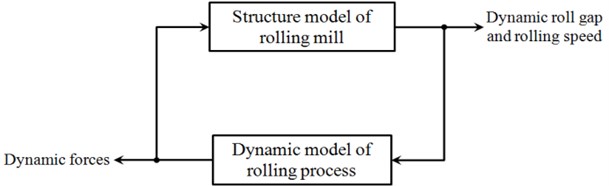
The current research generally considered that the mill vibration is a typical kind of self-excited vibration, which is the consequence of interactions between the system structure and the rolling process [3]. This interaction can be represented by the closed-loop shown in Fig. 1. The dynamic forces which are generated in the rolling process deflect the structure of the rolling mill and lead to variations of the roll gap and the rolling speed. These, in turn, result in further variations of the rolling forces. Therefore, simplifying the rolling process effectively and modeling the mill structure reasonably are the key problems to study the rolling mill vibration.

Fig. 1Coupling relationship of structure model and rolling process model

For the rolling process model, Yun et al. [4] and Hu et al. [5, 6] carried out a systematic research on its modeling. Based on Tlusty model [2], Yun et al. [4] presented a new dynamic rolling process model, in which the strip strain-hardening effect and the metal flow equation in the condition of vibration were taken into consideration. On this basis, Hu et al. [5] further modified the metal flow equation, and constructed a more accurate dynamic rolling process model. For the rolling mill structure model, different models were presented according to different research focuses and assumptions. The most typical structure models include vertical structure models (one degree of freedom [7], two degrees of freedom [7, 8] and four degrees of freedom [1]) and torsional structure models (single drive and twin drives) [9].

In actual production, vibrations of the high-speed rolling mill mostly appear as the coupling of multiple vibration types. Taking a two-high rolling mill as the object, Swiatoniowski [10] studied the interaction between the plastic deformation process and the rolling mill vibration, and constructed a typical vertical-torsional coupling structural model. Through experiments, Paton et al. [11] found that rolls can vibrate not only in vertical direction, but also in horizontal direction. Yan et al. [12] studied the coupling characteristic of torsional vibration and vertical vibration by the finite-element analysis.

Furthermore, many experiments and theoretical studies have shown that the lubrication condition in the roll bite is one of the most important factors affecting the rolling mill vibration. Yarita et al. [1] pointed out that lubrication defects may cause vibration, and better lubrication conditions can suppress vibration effectively. Based on the nonlinear friction model proposed by Sims and Arthur [13], Shi et al. [14] studied the stability of the rolling mill main drive system. Vladimir et al. [15] studied the vibration of a hot rolling mill with the consideration of the stick-slip nonlinear friction model [16], and indicated that frictional conditions along the contact arc were indeed the principal cause of the vibration in that rolling mill.

However, in the existing dynamic rolling process models, the friction coefficient was usually taken as a constant, which cannot fully display the complex friction characteristics of the real system. Therefore, it is necessary to study the rolling mill multiple-modal-coupling vibration based on the dynamic rolling process model with nonlinear friction considered.

Reference [17] has constructed a rolling mill vertical-torsional-horizontal coupled dynamic model with the consideration of nonlinear friction. In this paper, a brief introduction of this mathematical model is given at the beginning. On this basis, the system stability domain is determined and the Hopf bifurcation types at different bifurcation points are judged. Then, the changes of the system stability domain with different rolling process parameters are mainly discussed. And a mean relative sensitivity factor is defined to compare the effects of different parameters. The results can provide a theoretical basis for formulating a reasonable rolling schedule, and drawing up an effective control strategy as well.

2. Mathematical model

As Fig. 1 shows, a rolling mill vibration model can be formulated naturally as the result of interactions between the rolling mill structure and the rolling process. Therefore, in this section, dynamic models of the rolling mill structure and the rolling process will be introduced respectively, and then the mathematical model is constructed by coupling these two dynamic models.

2.1. Dynamic model of rolling mill structure

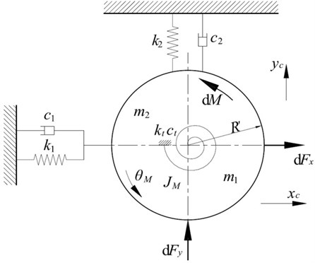
The vertical-torsional-horizontal coupled dynamic model of the rolling mill structure is illustrated in Fig. 2. In this structure model, the rolling mill is assumed to be symmetrical with respect to the center plane of the strip, and the vertical subsystem, horizontal subsystem and torsional subsystem are all simplified as ones with single degree of freedom.

Thus, the differential equations can be written as:

1

\{\begin{array}{l} m_{1} {\ddot{x}}_{c} + c_{1} {\dot{x}}_{c} + k_{1} x_{c} = d F_{x}, \\ m_{2} {\ddot{y}}_{c} + c_{2} {\dot{y}}_{c} + k_{2} y_{c} = d F_{y}, \\ J_{M} {\ddot{θ}}_{M} + c_{t} {\dot{θ}}_{M} + k_{t} θ_{M} = d M, \end{array}

where, $d F_{x}$ and $d F_{y}$ are fluctuations of forces acting on the rolls in $x$ and $y$ directions, $d M$ is the fluctuation of the rolling torque. The expressions of these three dynamic forces can be obtained in the dynamic model of the rolling process.

Fig. 2Simplified vertical-torsional-horizontal coupling structure model

2.2. Dynamic model of rolling process with nonlinear friction

For cold rolling, when the rolling speed is greater than 0.25 m·s^-1, the friction coefficient along the contact arc can be approximately expressed as [13]:

2

μ = a e x p (- b v_{r} + c),

where, $a$ , $b$ and $c$ are constants, which are related to lubricating oil viscosity, lubricating oil concentration and system lubricating state. And the values of $a$ , $b$ and $c$ are all greater than zero. $v_{r}$ is the work roll peripheral velocity. In this paper, the work roll is allowed to vibrate in vertical, horizontal and torsional directions, there into, both the horizontal vibration and the torsional vibration can affect the peripheral velocity of the work roll. Therefore, when vibration occurs, the expression of the work roll peripheral velocity is rewritten as: $v_{r} = {\bar{v}}_{r} + {\dot{θ}}_{M} R' + {\dot{x}}_{c}$ . ${\bar{v}}_{r}$ is the work roll peripheral velocity under steady state.

For convenience, the friction coefficient $μ$ near the steady roll peripheral velocity ${\bar{v}}_{r}$ has been deduced by Taylor series expansion:

3

μ = μ ({\bar{v}}_{r}) + μ' ({\bar{v}}_{r}) (v_{r} - {\bar{v}}_{r}) + \frac{μ'' ({\bar{v}}_{r})}{2} {(v_{r} - {\bar{v}}_{r})}^{2}

= a e^{- b {\bar{v}}_{r} + c} [1 - b ({\dot{θ}}_{M} R' + {\dot{x}}_{c}) + \frac{1}{2} b^{2} ({\dot{θ}}_{M} R' + {\dot{x}}_{c})^{2}]

= μ_{0} [1 - b ({\dot{θ}}_{M} R' + {\dot{x}}_{c}) + \frac{1}{2} b^{2} ({\dot{θ}}_{M} R' + {\dot{x}}_{c})^{2}],

where, $μ_{0}$ is the steady friction coefficient when the work roll peripheral velocity is ${\bar{v}}_{r}$ , $μ_{0} = a e x p (- b {\bar{v}}_{r} + c)$ .

Using Eq. (3) to represent the friction characteristic along the contact arc, the detailed derivation of the dynamic rolling process model with the consideration of nonlinear friction is given in Appendix A1 [17].

2.3. Dynamical equation of rolling mill vertical-torsional-horizontal coupled vibration

When constructing the dynamical equation of the rolling mill vibration, the inter-stand tension effect must be considered. As the vibration characteristic of a single stand rolling mill is the focus in this study, supposing the variations of both the exit velocity of the upstream stand and the entry velocity of the downstream stand are zero. Then the tension variations at entry and exit can be obtained according to Hooke’s law. That is:

4

\{\begin{array}{l} \frac{d (d σ_{0})}{d t} = \frac{E_{1}}{L_{0}} d v_{0}, \\ \frac{d (d σ_{1})}{d t} = - \frac{E_{1}}{L_{1}} d v_{1} . \end{array}

Substituting $(d F_{x}, d F_{y}, d M, d v_{0}, d v_{1})$ from Eq. (A11) into Eq. (1) and Eq. (4), the dynamical equation of the rolling mill vertical-torsional-horizontal coupled vibration can be expressed as:

5

\{\begin{array}{l} {\dot{x}}_{1} = x_{2}, \\ {\dot{x}}_{2} = \frac{1}{m_{1}} [- k_{1} x_{1} - c_{1} x_{2} + a_{F_{x}, y_{c}} x_{3} + a_{F_{x}, σ_{0}} x_{7} + a_{F_{x}, σ_{1}} x_{8} + a_{F_{x}, h_{0}} d h_{0}], \\ {\dot{x}}_{3} = x_{4}, \\ {\dot{x}}_{4} = \frac{1}{m_{2}} [\begin{array}{l} a_{F_{y}, {\dot{x}}_{c}} x_{2} + (a_{F_{y}, y_{c}} - k_{2}) x_{3} + (a_{F_{y}, {\dot{y}}_{c}} - c_{2}) x_{4} + a_{F_{y}, {\dot{θ}}_{M}} x_{6} + a_{F_{y}, σ_{0}} x_{7} \\ + a_{F_{y}, σ_{1}} x_{8} + a_{F_{y}, {\dot{x}}_{c}^{2}} x_{2}^{2} + a_{F_{y}, {\dot{θ}}_{M}^{2}} x_{6}^{2} + a_{F_{y}, {\dot{θ}}_{M} {\dot{x}}_{c}} x_{2} x_{6} + a_{F_{y}, h_{0}} d h_{0} \end{array}], \\ {\dot{x}}_{5} = x_{6}, \\ {\dot{x}}_{6} = \frac{1}{J_{M}} [\begin{array}{l} a_{M, {\dot{x}}_{c}} x_{2} + a_{M, y_{c}} x_{3} + a_{M, {\dot{y}}_{c}} x_{4} - k_{t} x_{5} + (a_{M, {\dot{θ}}_{M}} - c_{t}) x_{6} + a_{M, σ_{0}} x_{7} \\ + a_{M, σ_{1}} x_{8} + a_{M, {\dot{x}}_{c}^{2}} x_{2}^{2} + a_{M, {\dot{θ}}_{M}^{2}} x_{6}^{2} + a_{M, {\dot{θ}}_{M} {\dot{x}}_{c}} x_{2} x_{6} + a_{M, h_{0}} d h_{0} \end{array}], \\ {\dot{x}}_{7} = \frac{E_{1}}{L_{0}} [\begin{array}{l} a_{v_{0}, {\dot{x}}_{c}} x_{2} + a_{v_{0}, y_{c}} x_{3} + a_{v_{0}, {\dot{y}}_{c}} x_{4} + a_{v_{0}, {\dot{θ}}_{M}} x_{6} + a_{v_{0}, σ_{0}} x_{7} + a_{v_{0}, σ_{1}} x_{8} \\ + a_{v_{0}, {\dot{x}}_{c}^{2}} x_{2}^{2} + a_{v_{0}, {\dot{θ}}_{M}^{2}} x_{6}^{2} + a_{v_{0}, {\dot{θ}}_{M} {\dot{x}}_{c}} x_{2} x_{6} + a_{v_{0}, h_{0}} d h_{0} \end{array}], \\ {\dot{x}}_{8} = - \frac{E_{1}}{L_{1}} [\begin{array}{l} a_{v_{1}, {\dot{x}}_{c}} x_{2} + a_{v_{1}, y_{c}} x_{3} + a_{v_{1}, {\dot{y}}_{c}} x_{4} + a_{v_{1}, {\dot{θ}}_{M}} x_{6} + a_{v_{1}, σ_{0}} x_{7} + a_{v_{1}, σ_{1}} x_{8} \\ + a_{v_{1}, {\dot{x}}_{c}^{2}} x_{2}^{2} + a_{v_{1}, {\dot{θ}}_{M}^{2}} x_{6}^{2} + a_{v_{1}, {\dot{θ}}_{M} {\dot{x}}_{c}} x_{2} x_{6} + a_{v_{1}, h_{0}} d h_{0} \end{array}], \end{array}

where, $X = {(x_{1}, x_{2}, x_{3}, x_{4}, x_{5}, x_{6}, x_{7}, x_{8})}^{T} = {(x_{c}, {\dot{x}}_{c}, y_{c}, {\dot{y}}_{c}, θ_{M}, {\dot{θ}}_{M}, d σ_{0}, d σ_{1})}^{T}$ .

3. System stability analysis

3.1. Hurwitz algebraic criterion

Hurwitz algebraic criterion is an important method, using which bifurcation points can be calculated by an algebraic equation. In particular, it can be effectively applied to analyze Hopf bifurcation of the high-dimensional and complicated nonlinear system [18].

In order to study the effect of the nonlinear friction on the system stability, selecting parameter $b$ as the bifurcation parameter. Then, Eq. (5) is a function of $X$ and $b$ , $\dot{X} = f (X, b)$ . As the coordinate origin is the equilibrium point of the system, the Jacobian matrix at this point is as follows:

6

A (0, b) = {\frac{\partial f (X, b)}{\partial X}|}_{X_{0} = 0}

= [\begin{matrix} 0 & 1 & 0 & 0 & 0 & 0 & 0 & 0 \\ \frac{- k_{1}}{m_{1}} & \frac{- c_{1}}{m_{1}} & \frac{a_{F_{x}, y_{c}}}{m_{1}} & 0 & 0 & 0 & \frac{a_{F_{x}, σ_{0}}}{m_{1}} & \frac{a_{F_{x}, σ_{1}}}{m_{1}} \\ 0 & 0 & 0 & 1 & 0 & 0 & 0 & 0 \\ 0 & \frac{a_{F_{y}, {\dot{x}}_{c}}}{m_{2}} & \frac{a_{F_{y}, y_{c}} - k_{2}}{m_{2}} & \frac{a_{F_{y}, {\dot{y}}_{c}} - c_{2}}{m_{2}} & 0 & \frac{a_{F_{y}, {\dot{θ}}_{M}}}{m_{2}} & \frac{a_{F_{y}, σ_{0}}}{m_{2}} & \frac{a_{F_{y}, σ_{1}}}{m_{2}} \\ 0 & 0 & 0 & 0 & 0 & 1 & 0 & 0 \\ 0 & \frac{a_{M, {\dot{x}}_{c}}}{J_{M}} & \frac{a_{M, y_{c}}}{J_{M}} & \frac{a_{M, {\dot{y}}_{c}}}{J_{M}} & \frac{- k_{t}}{J_{M}} & \frac{a_{M, {\dot{θ}}_{M}} - c_{t}}{J_{M}} & \frac{a_{M, σ_{0}}}{J_{M}} & \frac{a_{M, σ_{1}}}{J_{M}} \\ 0 & \frac{E_{1} a_{v_{0}, {\dot{x}}_{c}}}{L_{0}} & \frac{E_{1} a_{v_{0}, y_{c}}}{L_{0}} & \frac{E_{1} a_{v_{0}, {\dot{y}}_{c}}}{L_{0}} & 0 & \frac{E_{1} a_{v_{0}, {\dot{θ}}_{M}}}{L_{0}} & \frac{E_{1} a_{v_{0}, σ_{0}}}{L_{0}} & \frac{E_{1} a_{v_{0}, σ_{1}}}{L_{0}} \\ 0 & \frac{- E_{1} a_{v_{1}, {\dot{x}}_{c}}}{L_{1}} & \frac{- E_{1} a_{v_{1}, y_{c}}}{L_{1}} & \frac{- E_{1} a_{v_{1}, {\dot{y}}_{c}}}{L_{1}} & 0 & \frac{- E_{1} a_{v_{1}, {\dot{θ}}_{M}}}{L_{1}} & \frac{- E_{1} a_{v_{1}, σ_{0}}}{L_{1}} & \frac{- E_{1} a_{v_{1}, σ_{1}}}{L_{1}} \end{matrix}] .

The characteristic equation of the Jacobian matrix can be obtained through calculating the determinant $|A (0, b) - λ I| = 0$ . Here, $I$ is an eight-order unit matrix:

7

λ^{8} + p_{1} λ^{7} + p_{2} λ^{6} + p_{3} λ^{5} + p_{4} λ^{4} + p_{5} λ^{3} + p_{6} λ^{2} + p_{7} λ + p_{8} = 0 .

A series of Hurwitz determinants can be constructed as follows:

8

Δ_{i} = |\begin{matrix} p_{1} & 1 & 0 & 0 & \dots & 0 \\ p_{3} & p_{2} & p_{1} & 1 & \dots & 0 \\ p_{5} & p_{4} & p_{3} & p_{2} & \dots & 0 \\ ⋮ & ⋮ & ⋮ & ⋮ & \dots & ⋮ \\ p_{2 i - 1} & p_{2 i - 2} & p_{2 i - 3} & p_{2 i - 4} & p_{i} \end{matrix}|,

here, $p_{i} =$ 0 when $i >$ 8.

For the system Hopf bifurcation to occur at point $b^{*}$ , the necessary and sufficient conditions judging by Hurwitz algebraic criterion should be satisfied:

9

\{\begin{array}{l} p_{i} (b^{*}) > 0, (i = 1,2, \dots, 8), \\ Δ_{7} (b^{*}) = 0, \\ Δ_{i} (b^{*}) > 0, (i = 5, 3, 1), \\ {\frac{d (Δ_{7} (b))}{d b}|}_{b = b^{*}} \neq 0 . \end{array}

3.2. Bifurcation parameter calculation and stability analysis

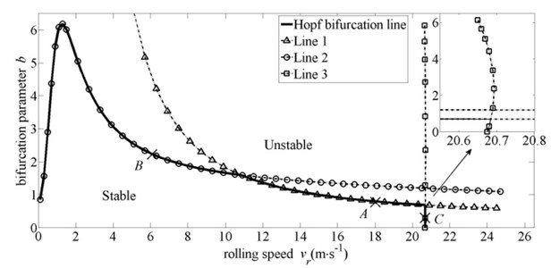
The simulation parameters used in this paper are from the 4th stand of a 2030 five-stand tandem cold rolling mill [19], and are listed in Table 1. Using these parameters, the distribution of Hopf bifurcation parameters with different steady rolling speeds is illustrated in Fig. 3. For this rolling mill, the frequencies of vertical vibration modal, torsional vibration modal and horizontal vibration modal are about 133 Hz, 12.5 Hz and 52 Hz, respectively.

From Fig. 3, it is observed that the system Hopf bifurcation line is spliced by Line 1, Line 2 and Line 3. Taking three points on these three lines randomly (point $A$ , point $B$ and point $C$ in Fig. 3), and their eigenvalues are listed in Table 2. Taking point $A$ as an example, when $b = 0.7982,$ a pair of pure imaginary eigenvalues appear in the system, $λ_{3,4} =$ (–0.0000±3.2682 $i$ )×10², and this pair of conjugate eigenvalues represent the characteristic of horizontal vibration modal, so Line 1 is the critical boundary of horizontal vibration modal. Similarly, Line 2 is the critical boundary of torsional vibration modal. Line 3 is the critical boundary of vertical vibration modal. And the system stability domain is enclosed by coordinate axes and the system Hopf bifurcation line.

Table 1Parameters from the 4th stand of a 2030 five-stand tandem cold mill

$m_{1}$ (kg)	$k_{1}$ (N·m^-1)	$c_{1}$ (N·s·m^-1)	${\bar{h}}_{0}$ (mm)	${\bar{h}}_{c}$ (mm)	$A$ (MPa)	$B$ (m)	$R$ (m)
9200	1×10⁹	5×10⁴	0.789	0.577	810	1.206	0.3
$m_{2}$ (kg)	$k_{2}$ (N·m^-1)	$c_{2}$ (N·s·m^-1)	${\bar{σ}}_{0}$ (MPa)	${\bar{σ}}_{1}$ (MPa)	$n$	$H$ (mm)	$R^{'}$ (m)
203200	6.9×10¹⁰	1.64×10⁷	180	189	0.29	2	0.5335
$J_{M}$ (kg·m²)	$k_{t}$ (N·m·rad^-1)	$c_{t}$ (N·m·s·rad^-1)	$L_{0}$ (m)	$L_{1}$ (m)	$E_{1}$ (GPa)	$μ_{0}$
1381	7.9×10⁶	4178	4.75	4.75	210	0.04

Table 2Eigenvalues about the critical parameters

$v_{r}$ (m·s^-1)	$b$		$λ_{1,2}$ (×10²)	$λ_{3,4}$ (×10²)	$λ_{5,6}$ (×10²)	$λ_{7}$ (×10²)	$λ_{8}$ (×10²)
18.0000	$A$ +	0.8200	–0.1815±8.3787 $i$	0.0008±3.2674 $i$	–0.0339±0.7868 $i$	–2.6399	–0.9583
	$A$	0.7982	–0.1816±8.3783 $i$	–0.0000±3.2682 $i$	–0.0355±0.7870 $i$	–2.6347	–0.9593
	$A$ -	0.7800	–0.1816±8.3779 $i$	–0.0007±3.2689 $i$	–0.0369±0.7871 $i$	–2.6303	–0.9601
6.0000	$B$ +	2.2700	–1.8620±8.0343 $i$	–0.0146±3.2511 $i$	0.0008±0.8035 $i$	–0.9738	–0.2893
	$B$	2.2541	–1.8622±8.0342 $i$	–0.0147±3.2515 $i$	–0.0000±0.8040 $i$	–0.9719	–0.2894
	$B$ -	2.2400	–1.8624±8.0341 $i$	–0.0148±3.2518 $i$	–0.0007±0.8046 $i$	–0.9703	–0.2895
20.6945	$C$ +	0.2885	0.0009±8.4145 $i$	–0.0182±3.2876 $i$	–0.0676±0.7824 $i$	–2.8762	–1.1455
20.6800	$C$		–0.0000±8.4143 $i$	–0.0182±3.2876 $i$	–0.0676±0.7824 $i$	–2.8742	–1.1447
20.6700	$C$ -		–0.0006±8.4141 $i$	–0.0182±3.2876 $i$	–0.0677±0.7825 $i$	–2.8729	–1.1441

In Fig. 3, there are three cross points on the curves, their abscissas are 10.9 m·s^-1, 20.684 m·s^-1 and 20.675 m·s^-1, respectively. These three cross points divide the system unstable domain into three regions. At the different regions, the system Hopf bifurcation induced by the variation of the friction coefficient could cause the system instability with different vibration modals.

Fig. 3The distribution of bifurcation parameter b* with steady rolling speed v-r

3.3. Hopf bifurcation type judgment

Hopf bifurcation can be classified as the super-critical bifurcation and the sub-critical bifurcation. As different types of Hopf bifurcation having different vibration characteristics, therefore, it is important to clear the Hopf bifurcation type at each bifurcation point.

Reference [20] defined a coefficient $η$ to judge the Hopf bifurcation type at different bifurcation points. The expression of the coefficient is:

10

η = R_{e} (- U f_{x x x} V V V^{*} + 2 U f_{x x} V A^{- 1} (0, b) f_{x x} V V^{*} + U f_{x x} V^{*} {(A (0, b) - 2 i ω_{0} I)}^{- 1} f_{x x} V V),

where:

f_{x x x} V V V^{*} = {(\frac{\partial}{\partial X} ((\frac{\partial}{\partial X} ((\frac{\partial f (X, b)}{\partial X}) V)) V)) V^{*}|}_{X = 0, b = b^{*}} .

The vector $U$ and the vector $V$ are the left eigenvector and the right eigenvector corresponding to the pure imaginary eigenvalues (± $ω_{0} i$ ) of the Jacobian matrix, that is $U A (0, b) = i ω_{0} U$ and $A (0, b) V = i ω_{0} V$ . Moreover, the vector $U$ and the vector $V$ also meet the condition $U V = 1$ . $V^{*}$ is the conjugate vector of the vector $V$ . $I$ is an eight-order unit matrix.

If $η > 0$ , the system Hopf bifurcation is the super-critical bifurcation. And when $η < 0$ , the system Hopf bifurcation is the sub-critical bifurcation.

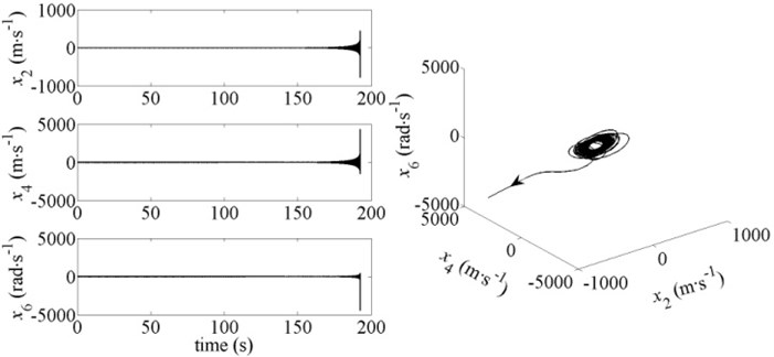
Substituting Hopf bifurcation points $A$ , $B$ and $C$ into Eq. (10), and the coefficient $η$ of each point is calculated. At point $A$ , $η =$ 3.72×10^-18 $>$ 0, it means that the system Hopf bifurcation at this point is the super-critical bifurcation. At point $B$ , $η =$ 5.39×10^-17 $>$ 0, and the system Hopf bifurcation at point $B$ is the super-critical bifurcation too. At point $C$ , $η =$ –3.01×10^-25 $<$ 0, the system Hopf bifurcation at this point is the sub-critical bifurcation.

Fig. 4Dynamic response and phase diagram of the system for v-r= 18 m∙s-1 and b= 0.82

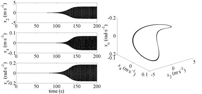
Fig. 5Dynamic response and phase diagram of the system for v-r= 6 m∙s-1 and b= 2.27

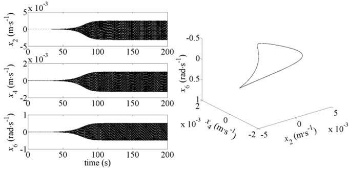
The system motions and three-dimensional phase diagrams in the period of 190-200 s corresponding to the point $A$ +, point $B$ + and point $C$ + are shown in Figs. 4-6. It can be seen that the system motions will form a stable limit-cycle eventually when the Hopf bifurcation occurs at point $A$ and point $B$ . But at point $C$ , the vibration amplitude is diverging over time when the Hopf bifurcation occurs, and the system will collapse within a short time. The simulation results shown in Figs. 4-6 are consistent with the results calculated by Eq. (10).

Through the analysis mentioned above, it can be seen that the system Hopf bifurcation curve is spliced by the critical boundaries of torsional vibration modal, horizontal vibration modal and vertical vibration modal. And for the different Hopf bifurcation points at different critical boundaries, the system Hopf bifurcation types may be different. Therefore, it is important and meaningful to study the movement laws of these three critical lines due to the change of rolling process parameters. And these laws can provide technical support for formulating a reasonable rolling process planning.

Fig. 6Dynamic response and phase diagram of the system for v-r= 20.6945 m∙s-1 and b= 2.2885

4. Effect of rolling process parameters on system stability domain

4.1. Tensions at entry and exit

The influences of tensions at entry and exit on the system stability domain are depicted in Fig. 7 and Fig. 8. There into, Fig. 7 is produced on the conditions of the entry tension equals to 0.75 $σ_{0}$ , $σ_{0}$ and 1.25 $σ_{0}$ , respectively, with other parameters unchanged. And Fig. 8 is produced on the conditions of the exit tension equals to 0.75 $σ_{1}$ , $σ_{1}$ and 1.25 $σ_{1}$ , respectively, with other parameters unchanged.

As shown in Fig. 7 and Fig. 8, with the increase of tensions at entry and exit, the critical boundary of vertical vibration modal moves left gradually, and the critical speed decreases accordingly. The reason is that larger tensions corresponding to the smaller rolling stiffness ( $a_{F y, y c}$ ). Thus the stability of vertical vibration modal reduces. For torsional vibration modal, the critical boundary moves down as the increase of the entry tension, and moves up as the increase of the exit tension. This is mainly due to the larger exit tension and the smaller entry tension mean the bigger forward slip zone. And the area difference between the size of the backward slip zone and the size of the forward slip zone becomes smaller. The rolling torque decreases accordingly. So the fluctuation of the rolling torque is relatively small with the same variations of the roll gap, and the torsional vibration modal is more stable. For horizontal vibration modal, its stability trend is the same with torsional vibration modal. The reason is that the larger exit tension and the smaller entry tension mean the force acting on the rolls in $x$ direction is smaller. Accordingly, the fluctuation of this force is smaller under the same disturbance, and the horizontal vibration modal is more stable.

Fig. 7Influence of entry tension on system stability domain

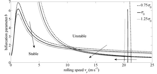
Fig. 8Influence of exit tension on system stability domain

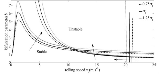
Fig. 9Influence of steady friction coefficient on system stability domain

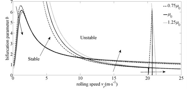
4.2. Steady friction coefficient

Fig. 9 represents the influence of the steady friction coefficient on the system stability domain. As Fig. 9 displays, the stability of the vertical subsystem is strengthened with the higher steady friction coefficient. The reason is that the friction in the roll gap acts as a positive damping in the vertical subsystem. For torsional vibration modal, as the increase of the steady friction coefficient, the modal is less stable at very low speeds, and more stable at medium and high speeds. On the one hand, the rolling torque increases as the increase of the steady friction coefficient, and the fluctuation of the rolling torque is greater under the same disturbance. On the other hand, the larger steady friction coefficient means the bigger forward slip zone, and the rolling torque decreases due to the increase of the forward slip zone, so the fluctuation of the rolling torque is smaller under the same disturbance. These two opposite trends play the dominant role alternately in different rolling speed stages. In the low-speed stage, the variation of the forward slip zone is relatively small. The first reason plays the dominant role at the moment. So the modal is less stable with the larger steady friction coefficient. With the continuous increase of the rolling speed, the second reason achieves the dominant role gradually, and the modal is more stable. For horizontal vibration modal, the fluctuation of the neutral point decreases with the increase of the steady friction coefficient. Accordingly, the variations of strip velocities as well as the variations of tensions are smaller. So the fluctuation of the force acting on the rolls in x direction is relatively smaller, and the modal is more stable.

4.3. Reduction ratio and strip thickness

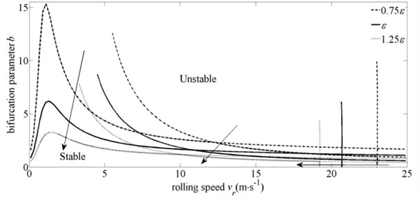
Since the functional relationship of the reduction ratio and strip thicknesses at entry and exit, the influences of the reduction ratio and strip thicknesses on the system stability domain are discussed in three different cases. The changes of the system stability domain with different reduction ratios are plotted in Fig. 10 and Fig. 11. There into, Fig. 10 considers the condition of invariable entry thickness, and Fig. 11 considers the condition of invariable exit thickness. In Fig. 12, the influence of the entry thickness on the system stability domain is displayed, in which the reduction ratio is kept unchanged.

As shown in Fig. 10 and Fig. 11, with the increase of the reduction ratio, all the critical boundaries move left or down, which mean the stabilities of all the modals are weakened. The reason is that the larger reduction ratio corresponds to the greater rolling torque and forces acting on the rolls in $x$ and $y$ directions. So, the fluctuations of these three forces increase with the same variations of the roll gap, and the emergence of the vibration is caused more easily.

Fig. 10Influence of reduction ratio on system stability domain with invariable entry thickness

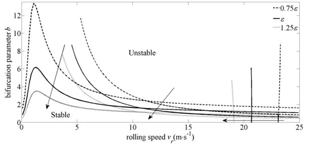
Fig. 11Influence of reduction ratio on system stability domain with invariable exit thickness

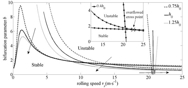
In Fig. 12, on the premise of the constant reduction ratio, with the increase of the strip entry thickness, the strip exit thickness increases simultaneously. For vertical vibration modal, Fig. 12 illustrates that the thicker the strip is, the more stable the modal will be. It is because that the thicker strip corresponds to relatively smaller volume variations of the strip under the same variations of the roll gap. So, the fluctuation of the force acting on the rolls in y direction decreases, accordingly. And the modal is more stable. But for torsional vibration modal and horizontal vibration modal, the stability trends are opposite to vertical vibration modal. For torsional vibration modal, the reason is that the increase of the entry thickness means the increasing length of the contact arc, so the area difference between the size of the backward slip zone and the size of the forward slip zone becomes bigger, and the rolling torque is larger accordingly. Therefore, the fluctuation of the rolling torque is relatively large with the same variations of the roll gap, so the modal stability is weakened. For horizontal vibration modal, the increase of strip thicknesses at entry and exit mean the increasing of the force acting on the rolls in $x$ direction. Thus, the fluctuation of this force increases with the same variations of the roll gap, so the modal is less stable.

Through further observation of Fig. 12, the cross point of the torsional critical boundary and the horizontal critical boundary moves to the right drastically as the decrease of the strip entry thickness. Therefore, it can be inferred that the cross point may overflow or disappear if the entry thickness continues to decrease. In other words, when rolling the thin strip, the whole system would not loss stability induced by horizontal vibration modal. The subgraph of Fig. 12 shows the situation of the cross point overflows, when the strip entry thickness is decreased to 0.4 $h_{0}$ .

Fig. 12Influence of entry thickness on system stability domain with invariable reduction ratio

5. Comparison of the effects

As the influences of rolling process parameters on the system stability domain are nonlinear, it is difficult to measure the effect of each parameter. In this section, a mean relative sensitivity factor is defined using the data in Fig. 7-Fig. 12. For the critical boundaries of horizontal vibration modal and torsional vibration modal (Line 1 and Line 2), this factor is obtained through adding together the ratios of the bifurcation parameters at the same abscissa. Since the critical boundary of vertical vibration modal (Line 3) is more sensitive to the rolling speed, therefore, this factor is obtained through adding together the ratios of the rolling speeds at the same ordinate. Even though this factor is not accurate, but it can be used to compare the effects of different parameters on the stability of different vibration modals. This factor is expressed as:

11

\{\begin{array}{l} Line 1, 2 : S (u) = \frac{1}{2 n} (\sum_{i = 1}^{n} |l n \frac{b_{i} (0.75 u)}{b_{i} (u)}| + \sum_{i = 1}^{n} |l n \frac{b_{i} (1.25 u)}{b_{i} (u)}|), (i = 1,2, \dots, n), \\ Line 3 : S (u) = \frac{1}{2 n} (\sum_{i = 1}^{n} |l n \frac{v_{r i} (0.75 u)}{v_{r i} (u)}| + \sum_{i = 1}^{n} |l n \frac{v_{r i} (1.25 u)}{v_{r i} (u)}|), (i = 1,2, \dots, n) . \end{array}

The mean relative sensitivity factors for the aforementioned parameters are given in Table 3. Among the parameters, the reduction ratio has the most significant influence on the stability of all three vibration modals. In addition, the influence of the entry thickness on horizontal vibration modal and the influences of tensions at entry and exit on torsional vibration modal are relatively larger. For vertical vibration modal, the entry thickness and tensions have the second most influence on modal stability.

In conclusion, the system stability domain is closely related to rolling process parameters. And the effect of the reduction ratio is the most significant. Moreover, the stability trends of these three modal with the change of the reduction ratio are the same. Therefore, in continuously rolling production, reasonable allocating the reduction ratio of each stand in a tandem mill is the key to ensure the rolling mill running smoothly and efficiently.

Table 3Mean relative sensitivity factors for the aforementioned parameters

Vibration modal		$S$ ( $σ_{0}$ )	$S$ ( $σ_{1}$ )	$S$ ( $μ_{0}$ )	$S$ ( $ε$ - $h_{0}$ )	$S$ ( $ε$ - $h_{1}$ )	$S$ ( $h_{0}$ )
Horizontal	Line 1	0.077	0.090	0.086	0.384	0.477	0.259
Torsional	Line 2	0.101	0.112	0.039	0.412	0.433	0.058
Vertical	Line 3	0.025	0.026	0.013	0.100	0.091	0.023

6. Conclusions

In this paper, based on the rolling mill vertical-torsional-horizontal coupled dynamic model with the consideration of the nonlinear friction, the system stability domain has been determined by the Hurwitz algebraic criterion. Then, the system Hopf bifurcation types have been judged. Finally, the influences of rolling process parameters on the system stability domain have been analyzed in detail. The following conclusions are drawn:

1) The system stability domain is enclosed by the instability critical boundaries of torsional vibration modal, horizontal vibration modal and vertical vibration modal. At different Hopf bifurcation points, the system Hopf bifurcation types may be different.

2) The critical boundaries will move with the change of rolling process parameters, which in turn change the system stability domain simultaneously. Among the parameters, the influence of the reduction ratio is the most significant. In addition to the reduction ratio, the stability of horizontal vibration modal is more sensitive to the strip entry thickness. The stability of torsional vibration modal is more sensitive to tensions at entry and exit. And the stability of vertical vibration modal is more sensitive to both tensions and the strip entry thickness.

3) When rolling the thin strip, the cross point of the torsional critical boundary and the horizontal critical boundary may overflow or disappear. In that situation, the instability of the whole system induced by horizontal vibration modal would not occur.

4) In actual production, clearing the movement trends of stability domain boundaries with the change of different rolling process parameters can provide a theoretical reference for optimizing the rolling process planning as well as selecting an optimal rolling process parameter to construct a state feedback controller.

References

Yarita I., Furukawa K., Seino Y. An analysis of chattering in cold rolling of ultrathin gauge steel strip. Transactions ISIJ, Vol. 18, Issue 1, 1978, p. 1-10.

Publisher
Tlusty J., Critchley S., Paton D. Chatter in cold rolling. Annals of the CIRP, Vol. 31, Issue 1, 1982, p. 195-199.

Publisher
Gao Z. Y., Zang Y., Zeng L. Q. Review of chatter in the rolling mills. Journal of Mechanical Engineering, Vol. 51, Issue 16, 2015, p. 87-105.

Publisher
Yun I. S., Wilson W. R. D., Ehmann K. F. Chatter in the strip rolling process. Part 1: dynamic model of rolling; Part 2: dynamic rolling experiments; Part 3: chatter model. Journal of Manufacturing Science and Engineering, Vol. 120, Issue 5, 1998, p. 330-348.

Publisher
Hu P. H., Ehmann K. F. A dynamic model of the rolling process. Part 1: homogeneous model; Part 2: inhomogeneous model. International Journal of Machine Tools and Manufacture, Vol. 40, Issue 1, 2000, p. 1-31.

Publisher
Hu P. H., Zhao H. Y., Ehmann K. F. Third-octave-mode chatter in rolling. Part 1: chatter model; Part 2: stability of a single-stand mill; Part 3: stability of a multi-stand mill. Proceedings of the Institution of Mechanical Engineers, Part B: Journal of Engineering Manufacture, Vol. 220, Issue 8, 2006, p. 1267-1303.

Publisher
Tamiya T., Furui K., Lida H. Analysis of chattering phenomenon in cold rolling. Proceedings of Science and Technology of Flat Rolled Products, International Conference on Steel Rolling, Tokyo, Vol. 2, 1980, p. 1191-1207.

Search CrossRef
Hu P. H., Ehmann K. F. Fifth octave mode chatter in rolling. Proceedings of the Institution of Mechanical Engineerings, Part B: Journal of Engineering Manufacture, Vol. 215, Issue 6, 2001, p. 797-809.

Publisher
Krot P. Nonlinear vibrations and backlashes diagnostics in the rolling mills drive trains. ENOC, Saint Petersburg, Russia, Vol. 30, Issue 6, 2008, p. 26-30.

Search CrossRef
Swiatoniowski A. Interdependence between rolling mill vibrations and the plastic deformation process. Journal of Materials Processing Technology, Vol. 61, Issue 4, 1996, p. 354-364.

Publisher
Paton D. L., Critchley S. Tandem mill vibration: its cause and control. Iron and Steel Making, Vol. 12, Issue 3, 1985, p. 37-43.

Search CrossRef
Yan X. Q., Shi C., Cao X., et al. Research on coupled vertical-torsion vibration of mill-stand of CSP mill. Journal of Vibration, Measurement and Diagnosis, Vol. 28, Issue 4, 2008, p. 377-381.

Search CrossRef
Sims R. B., Arthur D. F. Speed-dependent variables in cold strip rolling. Journal of Iron and Steel Institute, Vol. 172, Issue 3, 1952, p. 285-295.

Search CrossRef
Shi Peiming, Xia Kewei, Liu Bin, et al. Dynamics behaviors of rolling mill’s nonlinear torsional vibration of multi-degree-of-freedom main drive system with clearance. Journal of Mechanical Engineering, Vol. 48, Issue 17, 2012, p. 57-64.

Publisher
Panjkovic V., Gloss R., Steward J., et al. Causes of chatter in a hot strip mill: Observations, qualitative analyses and mathematical modelling. Journal of Materials Processing Technology, Vol. 212, Issue 4, 2012, p. 954-961.

Publisher
Thomsen J. J. Using fast vibrations to quench friction-induced oscillations. Journal of Sound and Vibration, Vol. 228, Issue 5, 1999, p. 1079-1102.

Publisher
Zeng L. Q., Zang Y., Gao Z. Y., et al. Stability analysis of the rolling mill multiple-modal-coupling vibration under nonlinear friction. Journal of Vibroengineering, Vol. 17, Issue 6, 2015, p. 2824-2836.

Search CrossRef
Gao Z. Y., Zang Y., Wu D. P. Hopf bifurcation and feedback control of self-excited torsion vibration in the drive system. Noise and Vibration Worldwide, Vol. 42, Issue 10, 2001, p. 68-74.

Publisher
Zou J. X., Xu L. J. Tandem Mill Vibration Control. Metallurgical Industry Press, Beijing, 1998.

Search CrossRef
Liu B., Liu S., Zhang Y. K., et al. Bifurcation control for electromechanical coupling vibration in rolling mill drive system based on nonlinear feedback. Journal of Mechanical Engineering, Vol. 46, Issue 8, 2010, p. 160-166.

Publisher

Cited by

Vibration Energy Coupling Behavior of Rolling Mills under Double Disturbance Conditions

Lidong Wang | Shen Wang | Xingdou Jia | Xiaoling Wang | Xiaoqiang Yan

(2023)

Stability of nonlinear vibrations induced by rolling force in a precise cold mill system

Chaofan Sun | Wu Zhao | Dan Huang | Hongbin Zhang

(2023)

Dynamic Amplitude-Frequency Characteristics of Vertical–Torsional Coupling System with Harmonic Response in Hot Tandem Mill

Lidong Wang | Xiaoqiang Yan | Xingdou Jia | Xiaoling Wang

(2022)

Bifurcation characteristics of torsional-horizontal coupled vibration of rolling mill system

Shuang Liu | Yatao Shi | Yunpeng Zhang | Meng Zong

(2017)

About this article

Received

18 October 2015

Accepted

12 February 2016

Published

31 March 2016

SUBJECTS

Chaos, nonlinear dynamics and applications

DOI

https://doi.org/10.21595/jve.2016.16569

Keywords

rolling mill

vertical-torsional-horizontal coupling vibration

nonlinear friction

stability

rolling process parameters

Acknowledgements

This study is supported by the National Natural Science Foundation of China (No. 51175035), the Ph.D. Programs Foundation of Ministry of Education of China (No. 20100006110024), the Beijing Higher Education Young Elite Teacher Project (No. YETP0367) and the Fundamental Research Funds for the Central Universities (No. FRF-BR-14-006A).

This is an open access article distributed under the Creative Commons Attribution License, which permits unrestricted use, distribution, and reproduction in any medium, provided the original work is properly cited.