Bifurcation and chaos for electromechanical coupling torsional vibration in rolling mill system driven by DC motor

Liu, Haoran; Liu, Jinjie; Liu, Fei; Zhu, Zhanlong; Wang, Kun; Liu, Shuang

doi:10.21595/jve.2016.16565

Journal of Vibroengineering

Browse Journal

Submit article

Published: 15 May 2016

Check for updates

Bifurcation and chaos for electromechanical coupling torsional vibration in rolling mill system driven by DC motor

Haoran Liu¹

Jinjie Liu²

Fei Liu³

Zhanlong Zhu⁴

Kun Wang⁵

Shuang Liu⁶

^{1, 3}School of Information Science and Engineering, Yanshan University, Qinhuangdao, China

^{1, 3}The Key Laboratory for Special Fiber and Fiber Sensor of Hebei Province, Yanshan University, Qinhuangdao, China

^{2, 4, 6}School of Electrical Engineering, Yanshan University, Qinhuangdao, China

⁵School of Science, Yanshan University, Qinhuangdao, China

Corresponding Author:

Jinjie Liu

Cite the article Download PDF

Downloads 1406

WoS Core Citations 1

CrossRef Citations 1

Abstract

Bifurcation and chaos for electromechanical coupling torsional vibration in rolling mill system driven by DC motor is studied in this paper. Considering the electromechanical devices under unsaturated magnetic circuit, the dynamical equation of electromechanical coupling vibration in rolling mill drive system is deduced by using the dissipation Lagrange equation. The equivalent low-dimensional bifurcation equation, which can reveal the influence of system parameters on the nonlinear dynamic characteristics, is obtained by reducing the dimensionality system using the method of Lyapunov-Schmidt reduction, and the static bifurcation characteristic is analyzed by using the singularity theory. The torsional rigidity of rotating shaft and harmonic excitation are chosen as the bifurcation parameters. Finally, the simulation is carried out with actual parameters, the bifurcation diagram, Poincare map and the maximum Lyapunov exponent are also given, which show the influence of bifurcation parameters on the chaotic motions of the system.

1. Introduction

With the rapid development of the industrial technology, the rolling mill equipment continues melting towards maximization, high speed, automation and high accuracy directions. Torsional vibration of the rolling mill main drive system will serious affect the normal work and cause the damage to the equipment [1-3]. Torsional vibration is usually caused by nonlinear dynamic behaviors such as bifurcation and chaos. So there is great practice and immediate significance to study the nonlinear dynamic characteristics of the electromechanical coupling system.

The torsional vibration of rotational system was simulated and tested based on different work theory, which provides the experimental basis for torsional vibration analysis and control [4-6]. The low frequency torsional gap in shafts provides a new idea for vibration control, the vibration suppression in a lumped torsional system using wave-absorption control with online computation of an imaginary wave-propagation system was discussed, and the theoretical analysis showed that smaller mass and larger spring stiffness of an imaginary system absorb vibration energy better [7]. The propagation of torsional wave in the shaft with periodically attached local resonators was studied and the effect of shaft material on the vibration attenuation in band gap was investigated in Ref. [8]. Considering the effect of the backlash nonlinear factor of the relative rotation nonlinear dynamic system, the high-dimensional torsional vibration global dynamical equation was established based on Lagrange equation, the bifurcation characteristic was analyzed and the effects of the parameters on the vibration were discussed [9]. Abstracting the rolling mill main drive system into two masses or multi-mass relative rotation system, the bifurcation and the chaos which may cause torsional vibration of system were studied [10, 11]. A nonlinear feedback controller was also proposed to control the Hopf bifurcation point and the stability of periodic solutions. Gustavsson R. K. et al. [12] analyzed the effects of unbalance magnetic pull on the transverse vibration characteristics of motor rotor system. Taking high frequency converting current of inverter power switches into consideration, the electromechanical coupling dynamic model of high speed grinding system was established, and the physical mechanism of higher harmonic electromechanical coupling vibration was revealed in Ref. [13]. Wang Xingyuan et al. [14, 15] dealed with the existence of both Hopf bifurcation and topological horseshoe for a novel finance chaotic system. Kobayashi T. et al. [16] studied the effect of slot combination on acoustic noise from induction motors. Considering the high harmonic in electricity, Wu Huimin et al. [17] analyzed the effect of electromagnetic stiffness on the inherent frequency. Considering the influence of distribution of salient pole on air-gap permeance, model of electromechanical coupling torsional vibration for the rotor system under electromagnetic excitation was established by Xu Jinyou et al. [18]. Taking the nonlinearity of the generator shaft and the interaction of mechanics and electrics in the generator sets into account, a transient model was obtained by combining Park equations and mechanics equations in et al. [19]. The Hopf bifurcation, period-doubling bifurcation and chaos were investigated with nonlinear mode and Floquet theory. Considering the electromechanical devices with unsaturated magnetic circuit, the dynamic behavior of the system is analyzed by P. Woafo [20, 21].

Up to now, there are few researches about the electrical parameters in rolling mill torsional vibration system driven by DC motor. In this Letter, a transmission system driven by DC motor is abstracted as two masses torsional vibration model. The nonlinear electromechanical coupling dynamical equation of transmission system is established considering the coupling effect of electrical parameters and mechanical parameters. The equivalent low dimensional bifurcation equation is obtained and the bifurcation characteristic is analyzed by using the singularity theory. Finally, numerical simulations were performed to study the influence of torsional rigidity and excitation amplitude on chaotic motion. These provide a theoretical basis for design and control of the electromechanical coupling transmission system which is widely used in practical engineering.

2. Electromechanical coupling torsional vibration system

The main drive system of rolling mill usually consists of motor, universal couplings and rollers. The method of lumped mass is adopted to abstract the rolling mill main drive system driven by DC synchronous motor into a two-mass relative rotation model.

Considering the rolling mill main drive system under the incentive of torsional rigidity and outside disturbance, the total kinetic and potential energy of the system can be described as:

1

E = \frac{1}{2} J_{1} θ_{1}^{2} + \frac{1}{2} J_{2} θ_{2}^{2},

2

U = \frac{1}{2} K (θ_{1} - θ_{2})^{2} .

Damping force is:

3

F_{1}^{c} = - C ({\dot{θ}}_{1} - {\dot{θ}}_{2}),

4

F_{2}^{c} = - C ({\dot{θ}}_{2} - {\dot{θ}}_{1}) .

Generalized torque is:

5

Q_{j} = \sum_{i = 1}^{2} F_{i}^{i} \frac{\partial θ_{i}}{\partial q_{j}}, (j = 1, 2),

where $q_{j}$ ( $j =$ 1, 2) is generalized coordinate. Substituting Eq. (3), Eq. (4) into Eq. (5), yields the generalized torque:

6

Q_{1} = (F_{1} + F_{1}^{c}) \frac{\partial θ_{1}}{\partial θ_{1}} + (F_{2} + F_{2}^{c}) \frac{\partial θ_{2}}{\partial θ_{1}} = F_{1} - C ({\dot{θ}}_{1} - {\dot{θ}}_{2}),

7

Q_{2} = (F_{1} + F_{1}^{c}) \frac{\partial θ_{1}}{\partial θ_{2}} + (F_{2} + F_{2}^{c}) \frac{\partial θ_{2}}{\partial θ_{2}} = F_{2} - C ({\dot{θ}}_{2} - {\dot{θ}}_{1}) .

Substituting Eq. (6), Eq. (7) into Lagrange equation:

8

\frac{d}{d t} \frac{\partial E}{\partial {\dot{φ}}_{i}} - \frac{\partial E}{\partial φ_{i}} + \frac{\partial U}{\partial {\dot{φ}}_{i}} = Q_{i}, (i = 1, 2) .

Yields:

9

\{\begin{array}{l} J_{1} {\ddot{θ}}_{1} + K (θ_{1} - θ_{2}) + C ({\dot{θ}}_{1} - {\dot{θ}}_{2}) = F_{1}, \\ J_{2} {\ddot{θ}}_{2} - K (θ_{1} - θ_{2}) - C ({\dot{θ}}_{1} - {\dot{θ}}_{2}) = F_{2}, \end{array}

where $J_{1}$ and $J_{2}$ are inertia moments of the motor and mill roll, $θ_{i}$ and ${\dot{θ}}_{i}$ ( $i =$ 1, 2) are rotational angle and the speed of the rotational angle of motor and mill roll, $K$ is linear torsional stiffness of the system, $C$ is structural damping of the system, $F_{1}$ is output torque, $F_{2}$ is the damping force.

During the functioning of the devices, nonlinearity appears in the components of the mechanical parts. Indeed, for hardening torsion or compression effects in mechanical problems, the stiffness is not constant but increases with the applied constraint. The coefficient of torsion or compression can be approximated by the relation:

10

K = k_{l} + k_{n l} {(\frac{θ_{1}}{\partial_{0}})}^{2} = k_{l} [1 + δ {(\frac{θ_{1}}{\partial_{0}})}^{2}],

where $k_{l}$ is the stiffness for small torsion or compression, $θ_{1}$ is the rotation angle displacement, $δ$ is the coefficient of nonlinearity and $\partial_{0}$ is the normalization angle, the motor has two parts: a stator or inductor in a permanent magnet and a rotor, mobile around a revolution axis. To avoid the Foucault effect and to decrease the hysteresis loss, the following assumptions are considered: symmetrical magnetic circuit, negligible magnetic hysteresis, negligible magnetic flux leak [22]. Using Kirchhoff’s law, the equation of the electrical part is given by the following relation:

11

u (t) = R i + L \frac{d i}{d t} + K_{E} \frac{d θ_{1}}{d t},

where, in the right, the first term is the ohmic voltage, the second term is the voltage across the inductor, and the third term $K_{E} d θ_{1} / d t$ represents the coupling term between the electrical and mechanical parts. Using the Newton second law of dynamics for rotational motions and taking into account the Laplace force, the equation of the mechanical part is obtained as:

12

J_{Δ r} \frac{d^{2} θ_{1}}{d t^{2}} = - C_{v} \frac{d θ_{1}}{d t} + K_{T} i + T_{r},

where $J_{Δ r}$ is the moment of inertia of the rotor, $T_{v} = - C_{v} d θ_{1} / d t$ is the torque force due to viscous frictions, $K_{T}$ is the torque constant, $K_{T} i$ is the electromagnetic torque due to the Laplace force, $T_{r}$ is the resistive torque, it is modeled by the relation:

13

T_{r} = - K θ_{1} = - C_{r} [1 + δ {(\frac{θ_{1}}{\partial_{0}})}^{2}] θ_{1} = K_{1} θ_{1} + K_{2} {θ_{1}}^{3} .

When $F_{1} = K_{T} i$ and $F_{2} = T_{r}$ the system equations based on DC drive is:

14

\{\begin{array}{l} J_{1} {\ddot{θ}}_{1} + K (θ_{1} - θ_{2}) + C ({\dot{θ}}_{1} - {\dot{θ}}_{2}) = K_{T} i, \\ J_{2} {\ddot{θ}}_{2} - K (θ_{1} - θ_{2}) - C ({\dot{θ}}_{1} - {\dot{θ}}_{2}) = K_{1} θ_{1} + K_{2} θ_{1}^{3}, \\ R i + L \frac{d i}{d t} + K_{E} \frac{d θ_{1}}{d t} = u (t) . \end{array}

Eq. (14) is the nonlinear dynamic equation considering the torsional rigidity and the coupling term between the electrical and mechanical parts. In the process of motor running, $K_{1}$ is influenced by the motor load, the power supply voltage and the current. $K_{1}$ is selected as a major parameter to analyze the system dynamic characteristics in the following.

3. Bifurcation analysis of high dimensional electromechanical coupling system

If we want to analyze system characteristics the first step is dimensionless the data processing. In this paper, we use linear dimensionless method for data processing, assuming that the original data $x$ and dimensionless data $X$ have a linear relationship:

X = x U,

where $U$ is the dimensional scale, according to the practical parameters of electromechanical coupling torsional vibration system for 2150 rolling mill in a certain factory, a dimensionless form of linear proportional method is obtained by letting:

t^{*} = \frac{ω}{Ω} t, x_{1} = \frac{θ_{1}}{θ_{c}}, x_{2} = {\dot{x}}_{1}, x_{3} = \frac{θ_{2}}{θ_{c}}, x_{4} = {\dot{x}}_{3}, x_{5} = i, - \frac{K Ω^{2}}{J_{1} ω^{2}} = a, - \frac{C Ω}{J_{1} ω} = b,

\frac{K Ω^{2}}{J_{1} ω^{2}} = c, \frac{C Ω}{J_{1} ω} = d, \frac{K_{T} Ω^{2}}{J_{1} ω^{2}} = e, \frac{(K + K_{1}) Ω^{2}}{J_{2} ω^{2}} = g, \frac{C Ω}{J_{2} ω} = h, - \frac{K Ω^{2}}{J_{2} ω^{2}} = m, - \frac{C Ω}{J_{2} ω} = n,

\frac{K_{2} θ_{c}^{2} Ω^{2}}{J_{2} ω^{2}} = p, - \frac{K_{E} Ω}{L ω} = s, - \frac{R Ω}{L ω} = z, T = \frac{u (t)}{L},

where $ω / Ω$ is system dimensionless ratio value, $θ_{c}$ is standard reduced value for the system angle.

Considering the excitation amplitude of $F$ is added at the load equipment, Then Eq. (14) can be reduced order for first-order equation as follows:

15

\{\begin{array}{l} {\dot{x}}_{1} = x_{2}, \\ {\dot{x}}_{2} = a x_{1} + b x_{2} + c x_{3} + d x_{4} + e x_{5}, \\ {\dot{x}}_{3} = x_{4}, \\ x_{4} = g x_{1} + h x_{2} + m x_{3} + n x_{4} + p x_{1}^{3} + F, \\ {\dot{x}}_{5} = s x_{2} + z x_{5} . \end{array}

3.1. Lyapunov Schmidt reduction

Eq. (15) can be expressed as:

16

\dot{X} = f (X),

where $X = (x_{1}, x_{2}, x_{3}, x_{4}, x_{5})^{T}$ is the state variables of dynamic system and $f (X) = (f_{1}, f_{2}, f_{3}, f_{4}, f_{5})^{T}$ are the corresponding nonlinear vector functions.

At the equilibrium point $\bar{X}$ , system Eq. (16) satisfies:

17

f (\bar{X}) = 0 .

Let $D f (\bar{X})$ be the Jacobian matrix of $f (X)$ at the equilibrium:

18

D f (\bar{X}) = (\begin{array}{l} \frac{\partial f_{1}}{\partial x_{1}} & \frac{\partial f_{1}}{\partial x_{2}} & \frac{\partial f_{1}}{\partial x_{3}} & \frac{\partial f_{1}}{\partial x_{4}} & \frac{\partial f_{1}}{\partial x_{5}} \\ \frac{\partial f_{2}}{\partial x_{1}} & \frac{\partial f_{2}}{\partial x_{2}} & \frac{\partial f_{2}}{\partial x_{3}} & \frac{\partial f_{2}}{\partial x_{4}} & \frac{\partial f_{2}}{\partial x_{5}} \\ \frac{\partial f_{3}}{\partial x_{1}} & \frac{\partial f_{3}}{\partial x_{2}} & \frac{\partial f_{3}}{\partial x_{3}} & \frac{\partial f_{3}}{\partial x_{4}} & \frac{\partial f_{3}}{\partial x_{5}} \\ \frac{\partial f_{4}}{\partial x_{1}} & \frac{\partial f_{4}}{\partial x_{2}} & \frac{\partial f_{4}}{\partial x_{3}} & \frac{\partial f_{4}}{\partial x_{4}} & \frac{\partial f_{4}}{\partial x_{5}} \\ \frac{\partial f_{5}}{\partial x_{1}} & \frac{\partial f_{5}}{\partial x_{2}} & \frac{\partial f_{5}}{\partial x_{3}} & \frac{\partial f_{5}}{\partial x_{4}} & \frac{\partial f_{5}}{\partial x_{5}} \end{array}) .

The Lyapunov stability is decided by the eigenvalues of $D f (\bar{X})$ . The Jacobian matrix $D f (\bar{X})$ can be expressed as:

19

D f (\bar{X}) = (\begin{matrix} 0 & 1 & 0 & 0 & 0 \\ a & b & c & d & e \\ 0 & 0 & 0 & 1 & 0 \\ g + 3 p x_{1}^{2} & h & m & n & 0 \\ 0 & s & 0 & 0 & z \end{matrix}) .

This is a 5×5 square matrix and the value of the determinant is:

20

d e t (L) = λ^{5} + (- n - z - b) λ^{4} + (n z + b z + b n - h d - s e - a - m) λ^{3}

+ (h d z + a n - b n z + a z + b m + m z + s e n - h c - g d - 3 p d x_{1}^{2}) λ^{2}

+ (a m + h c z - a n z - b m z + s m e - g c + g d z - 3 p c x_{1}^{2} + 3 p d z x_{1}^{2}) λ

+ g c z + 3 p c z x_{1}^{2} - a m z = 0 .

There is a zero eigenvalue when $g c z + 3 p c z x_{1}^{2} - a m z = 0$ , and $L$ is a singular matrix.

It can be known that $d i m N (L) =$ 1, let $v_{0}$ be a basis vector of null space $N (L)$ , then we can get $v_{0} = (- c / a, 0,1, 0,0)$ . The adjoint operator of $L$ is the conjugate transpose matrix $L^{*}$ . Because $L$ is a real matrix and the conjugate transpose matrix $L^{*}$ is also a real matrix, and there is $L^{*} = L^{T}$ . We can see that $d i m N (L^{*}) =$ 1 since $L$ is a Fredholm operator with zero index. One basis vector:

v_{1} = (\frac{b q}{a} - \frac{q s e}{a z} - h, - \frac{q}{a}, \frac{d q}{a} - n, 1, - \frac{e q}{a z}),

of $d i m N (L^{*}) =$ 1 is obtained by calculation, where $q = g + 3 p {x_{1}}^{2}$ . So the five-dimensional Euclid space $R^{5}$ can be decomposed as follows:

R^{5} = N (L) \oplus M = R (L) \oplus N (L^{*}) .

Define the projection operator:

P : R^{5} \to R (L),

and the complementary projection operator:

I - P : R^{5} \to N (L^{*}) = s p a n \{v_{1}\},

then the equation:

21

f (x, p) = 0,

equivalent to:

22

\{\begin{array}{l} P f (v + w, p) = 0, \\ (I - P) f (v + w, p) = 0, \end{array}

where $v \in N (L) = s p a n (v_{0})$ , $w \in M$ . According to the definition of inner product in Euclid space, $(I - P) f (v + w, p) = 0$ is equivalent to:

23

〈 f (v + w, p), v_{1} 〉 = 0 .

Thus, the following equation is obtained:

24

(g + a) (\frac{b q}{a} - \frac{e s q}{a z} - h) + p {(\frac{b q}{a} - \frac{e s q}{a z} - h)}^{3} - \frac{q}{a} (1 + b + h + s)

+ (c + m) (\frac{d q}{a} - n) + \frac{e q}{a z} (e + z) + 1 + d + n + F = 0 .

Since $g c z + 3 p c z x_{1}^{2} - a m z = 0$ , rewritten this equation and substitute it into Eq. (24), then the expression of $x_{1}$ can be got:

25

A x_{1}^{6} + B x_{1}^{4} + C x_{1}^{2} + D = 0,

where:

A = p {(\frac{3 b p}{a} - \frac{3 p s e}{a z})}^{3}, B = 3 p (\frac{b g}{a} - \frac{s e g}{a z} - h) {(\frac{3 b p}{a} - \frac{3 p s e}{a z})}^{2} - 3 p (\frac{3 b p}{a} - \frac{3 p s e}{a z}),

C = \frac{3 p d (c + m)}{a} + 3 p (\frac{3 b p}{a} - \frac{3 p s e}{a z}) {(\frac{b g}{a} - \frac{s e g}{a z} - h)}^{2} + (a + \frac{a m}{c}) (\frac{3 b p}{a} - \frac{3 p s e}{a z})

- 3 p (\frac{b g}{a} - \frac{s e g}{a z} - h) - 3 \frac{p}{a} (1 + b + h + s) + \frac{3 p e (e + z)}{a z},

D = (\frac{a m}{c} + a) (\frac{b g}{a} - \frac{s e g}{a z} - h) + p {(\frac{b g}{a} - \frac{s e g}{a z} - h)}^{3} + (c + m) (\frac{d g}{a} - n)

- \frac{g (1 + b + h + s)}{a} + \frac{e g (e + z)}{a z} + d + n + 1 + F .

Assuming that a new state variable is $r = x_{1}$ , then the bifurcation equation can be written as:

26

G = r^{6} + α_{1} r^{4} + α_{2} r^{2} + β,

where $α_{1}$ , $α_{2}$ as the open fold parameters of bifurcation equation are both for the physical parameters of the system.

3.2. Singularity analysis

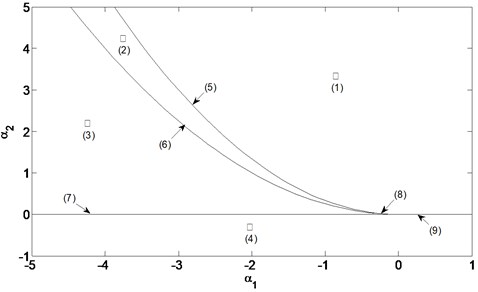
The topology of Eq. (26) and the effects of the open fold parameters on the bifurcation behavior will be studied by using the singularity theory. The following point sets are obtained based on the definition of the transition set:

I: Bifurcation point set:

B = \{(α_{1}, α_{2})| G = G_{r} = G_{β} = 0\} = Φ .

II: Lag point sets:

H_{1} = \{((α_{1}, α_{2}))| G = G_{r} = G_{r r} = 0\} = \{(α_{1}, α_{2})| α_{2} = 0\},

H_{2} = \{((α_{1}, α_{2}))| G = G_{r} = G_{r r} = 0\} = \{(α_{1}, α_{2}) | α_{2} = \frac{α_{1}^{2}}{3}, α_{1} \leq 0\} .

III: Bilimits point set:

D = \{((α_{1}, α_{2}))| G = G_{r} = 0\} = \{(α_{1}, α_{2}) | α_{2} = \frac{α_{1}^{2}}{4}, α_{1} \leq 0\} .

IV: Transition set:

\sum = H_{1} \cup H_{2} \cup D .

Transition set $\sum$ is shown in Fig. 1, the unfolding parametric space $α_{1} - α_{2}$ is divided into four subregions (I, II, III, IV) by $\sum$ and Eqs. (5)-(9) are bifurcation response curves of $\sum$ . Each subregion and its boundary bifurcation are shown in Fig. 2, Through the analysis of Fig. 2 we can draw the conclusion that: the roots of the Eq. (26) are smooth distribution in subregion I, the roots of the Eq. (26) have amplitude jump in subregion 2-9, This means that the system is not stable and such situations should be avoided in system designing and controlling.

Fig. 1Transition set

4. Numerical simulations of chaotic processes

As harmonic excitation often occurs torsional vibration in the process of the motor operation, and the harmonic excitation is not a fixed value, but cyclical changes over time, by Fourier transform it generally expressed as a linear combination of trigonometric functions (sine/cosine) or their integration. This paper adopts $F = f c o s (w t)$ for harmonic excitation, it is the general expression. In order to study the dynamic chaos of electromechanical coupling system, Runge-Kutta method is used for numerical simulation of torsion vibration system. Then Eq. (15) can be expressed as:

27

\{\begin{array}{l} {\dot{x}}_{1} = x_{2}, \\ {\dot{x}}_{2} = a x_{1} + b x_{2} + c x_{3} + d x_{4} + e x_{5}, \\ {\dot{x}}_{3} = x_{4}, \\ x_{4} = g x_{1} + h x_{2} + m x_{3} + n x_{4} + p x_{1}^{3} + f c o s (w t), \\ {\dot{x}}_{5} = s x_{2} + z x_{5} . \end{array}

Fig. 2Bifurcation diagram

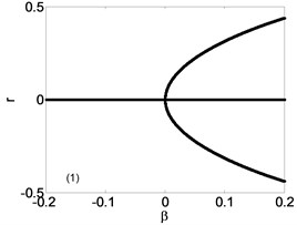
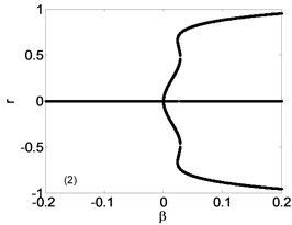
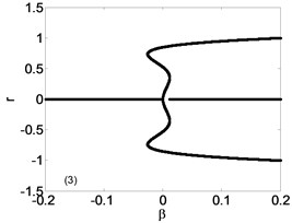
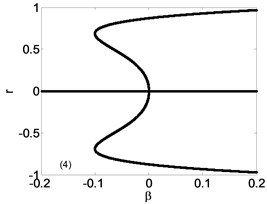
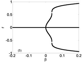
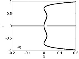
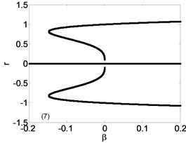
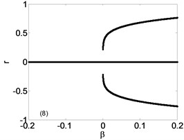
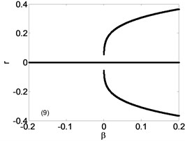
Fig. 3Bifurcation diagram in K1

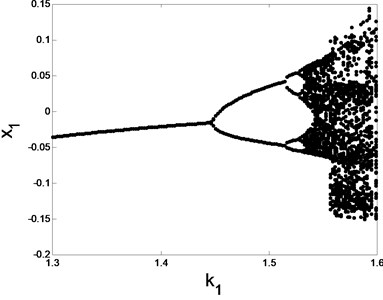
Fig. 4The maximum Lyapunov exponent

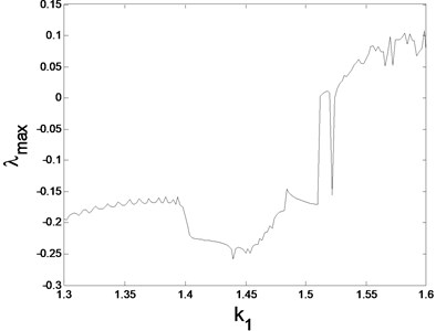
The system parameters can be taken as $a =$ –1.5, $b =$ –0.2, $c =$ 1.5, $d =$ 0.2, $e =$ 1.4, $h =$ 2, $m =$ –15, $n =$ –2, $p =$ –22, $s =$ –1.5, $z =$ –0.575, $w =$ 1 through dimensionless. The influence of torsional rigidity $K_{1}$ and excitation amplitude $f$ on electromechanical coupling system is discussed separately in this section. Take $f =$ 1.54 and with other parameters constant, while $K_{1}$ change in a wide range. The bifurcation diagrams and the maximum Lyapunov exponent of $K_{1}$ are shown in Fig. 3 and Fig. 4. It shows that system jumps into chaotic motion from a stable periodic motion with the increase of $K_{1}$ .

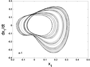
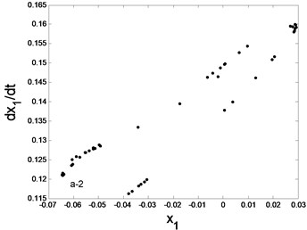
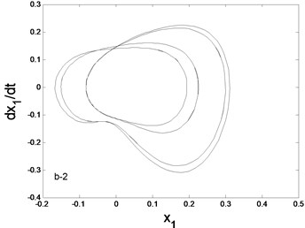
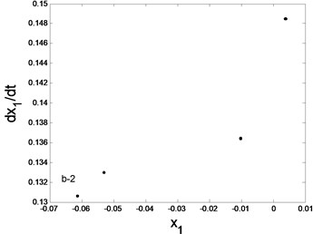
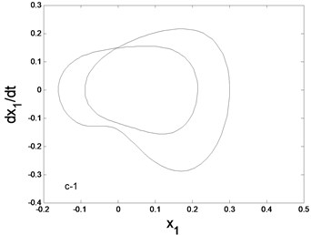
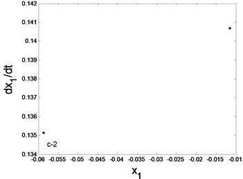
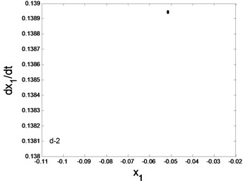
Fig. 5Phase trajectory (–1), Poincare map (–2) for different K1: a) K1= 1.4: b) K1= 1.5, c) K1= 1.52, d) K1= 1.58

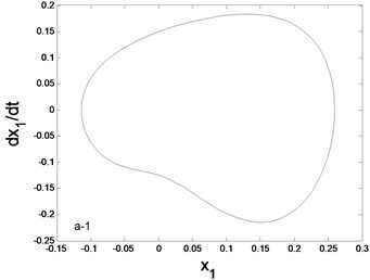
a1) Phase trajectory

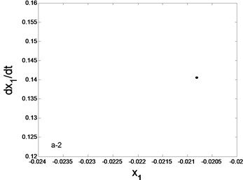
a2) Poincare map

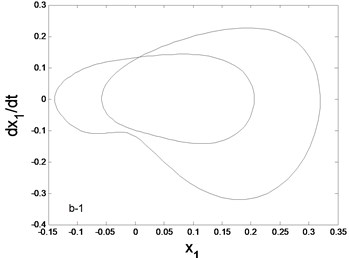
b1) Phase trajectory

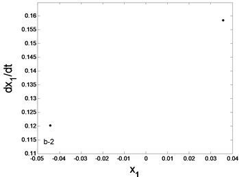
b2) Poincare map

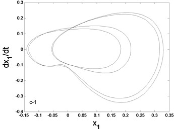
c1) Phase trajectory

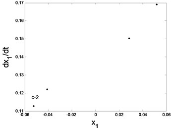
c2) Poincare map

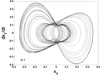
d1) Phase trajectory

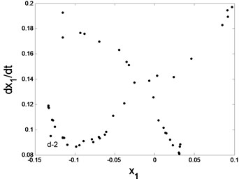
d2) Poincare map

The system phase diagrams and Poincare maps diagram under different $K_{1}$ are shown in Fig. 5. From Fig. 3, we can see that the bifurcation diagram changed when $K_{1} =$ 1.4, $K_{1} =$ 1.5 and $K_{1} =$ 1.52, system response is a stable periodic motion. It can be seen from Fig. 5(a)-(c) that the phase trajectory is a closed curve and the Poincare map has finite fixed points. From Fig. 4, the maximum Lyapunov exponent is greater than zero when $K_{1} =$ 1.58, it can be convincing of occurrence of chaotic motion. We can also see that phase trajectory repeatedly winding in enclosed area but not closed, and Poincare map has the obvious fractal structure from Fig. 5(c1), (c2).

When $K_{1} =$ 1.56 and keeps the other parameters constant, let $f$ change in a wide range. From the bifurcation diagram (Fig. 6.) and the maximum Lyapunov exponent (Fig. 7.) of $f$ , it can be seen that system jumps into single periodic motion from chaotic motion with the increase of $f$ .

Fig. 6Bifurcation diagram in f

Fig. 7The maximum Lyapunov

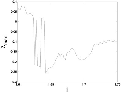
The system phase diagrams and Poincare maps with different $f$ are shown in Fig. 8 From Fig. 7, the maximum Lyapunov exponent is greater than zero when $f = 1.6$ , and the system appears chaotic motion. We can also see that phase trajectory repeatedly winding in enclosed area but not closed, and the Poincare map has the obvious fractal structure from Fig. 8(a). From Fig. 7, the maximum Lyapunov exponent is lower than zero when $f =$ 1.63, $f =$ 1.65 and $f =$ 1.7, system response appears a stable periodic motion. Then Fig. 8(b)-(d) show that phase trajectory is a closed curve, and Poincare map for a finite number of fixed points.

According to the numerical simulation, we come to a conclusion that both reducing torsional rigidity and increasing excitation amplitude can control the system from chaotic motion into stable periodic motion.

In order to control the chaotic motion, the external torque $T$ is introduced, assuming that kinetic equation with external torque $T$ is:

{\dot{x}}_{i} (t) = f_{i} (x, t) + T .

The original chaotic motion will be changed and the new stable periodic motion will appear when we adjust the external torque $T$ . The external torque $T$ must be kept in non-zero value after the system movement is driven to the stable periodic motion, at this moment we can achieve the goal of chaos control. The value range of $T$ can be determined according to the Lyapunov stability theory and adjusting the Lyapunov index size.

In this paper the external torque $T$ is joined when the system appears chaotic motion, and we can select the appropriate torque force to control chaotic motion through analyzing the system bifurcation diagram and the maximum Lyapunov exponent when the torque changes. This method does not need to know the stable periodic orbit and state variables of the system. It only needs to load the system’s motion to the periodic motion, by using the external torque, this method is simple and has little influence on the system's motor parameters.

Fig. 8Phase trajectory (–1), Poincare map (–2) for different f: a) f= 1.6, b) f=1.63, c) f=1.65, d) f= 1.7

a1) Phase trajectory

a2) Poincare map

b1) Phase trajectory

b2) Poincare map

c1) Phase trajectory

c2) Poincare map

d1) Phase trajectory

d2) Poincare map

5. Conclusions

In this paper, considering the electromechanical devices with unsaturated magnetic circuit, a high dimensional dynamical equation of electromechanical coupling vibration in rolling mill drive system are deduced by using the dissipation Lagrange equation. The equivalent low-dimensional bifurcation equation which can reveal the influence of system parameters on the nonlinear dynamic characteristics is obtained by reducing the dimensionality of the system. The static bifurcation is studied by using the singularity theory. Considering outside incentive, choose $K_{1}$ and $f$ are chosen as bifurcation parameters, Numerical simulations are also given at last, which show that both reducing torsional rigidity and increasing excitation amplitude can control the system from chaotic motion into stable periodic motion, we can also add a constant torque direct feedback method to control chaos. These results have an important theoretical significance on reducing the vibration of electromechanical coupling transmission system. In addition, the research in our paper provides a reference for the real design of motor’s parameters of electromechanical coupling transmission system.

References

Polat A. The effects of strain rate and temperature on the deformation behavior of cold-rolled TRIP800 steel. Steel Research International, Vol. 83, Issue 8, 2012, p. 775-782.

Publisher
Barrales-Mora L. A., Lü Y., Molodov D. A. Experimental determination and simulation of annealing textures in cold rolled TWIP and TRIP steels. Steel Research International, Vol. 82, Issue 2, 2011, p. 119-126.

Publisher
Amer Y. A., El-Sayed A.-T., El-Bahrawy F.-T. Torsional vibration reduction for rolling mill’s main drive system via negative velocity feedback under parametric excitation. Journal of Mechanical Science and Technology, Vol. 29, Issue 4, 2015, p. 1581-1589.

Publisher
Xiang L., Yang S., Gan C. Torsional vibration measurements on rotating shaft system using laser Doppler vibrometer. Optics and Lasers in Engineering, Vol. 50, Issue 11, 2012, p. 1596-1601.

Publisher
Wenzhi G., Zhiyong H. Active control and simulation test study on torsional vibration of large turbo-generator rotor shaft. Mechanism and Machine Theory, Vol. 45, Issue 9, 2010, p. 1326-1336.

Publisher
Kim H., Park C. I., Lee S. H., et al. Non-contact modal testing by the electromagnetic acoustic principle: applications to bending and torsional vibrations of metallic pipes. Journal of Sound and Vibration, Vol. 332, Issue 4, 2013, p. 740-751.

Publisher
Saigo M., Tanaka N., Nam D. H. Torsional vibration suppression by wave-absorption control with imaginary system. Journal of Sound and Vibration, Vol. 270, Issue 4, 2004, p. 657-672.

Publisher
Yu D., Liu Y., Wang G., et al. Low frequency torsional vibration gaps in the shaft with locally resonant structures. Physics Letters A, Vol. 348, Issue 3, 2006, p. 410-415.

Publisher
Liu S., Liu B., Shi P. M. Nonlinear feedback control of Hopf bifurcation in a relative rotation dynamical system. Acta Physica Sinica, Vol. 58, Issue 7, 2009, p. 4383-4389.

Publisher
Shi P. M., Liu B., Hou D. X. Global dynamic characteristic of nonlinear torsional vibration system under harmonically excitation. Chinese Journal of Mechanical Engineering, Vol. 22, Issue 1, 2009, p. 132-139.

Publisher
Liu S., Li X., Zhao S., et al. Bifurcation and chaos analysis of a nonlinear electromechanical coupling transmission system driven by AC asynchronous motor. International Journal of Applied Electromagnetics and Mechanics, Vol. 47, Issue 3, 2015, p. 705-717.

Publisher
Gustavsson R. K., Aidanpää J. O. The influence of nonlinear magnetic pull on hydropower generator rotors. Journal of Sound and Vibration, Vol. 297, Issue 3, 2006, p. 551-562.

Publisher
Lu L., Xiong W. L., Hou Z. Q. Research on match characteristics of a motorized spindle system to suppress electromechanical coupling vibration. Chinese Journal of Mechanical Engineering, Vol. 48, Issue 9, 2012, p. 144-154.

Publisher
Wang X. Y., Liang Q. Y., Meng J. Chaos and fractals in C-K map. International Journal of Modern Physics C, Vol. 19, Issue 9, 2011, p. 1389-1409.

Publisher
Ma C., Wang X. Y. Hopf bifurcation and topological horseshoe of a novel finance chaotic system. Communications in Nonlinear Science and Numerical Simulation, Vol. 17, Issue 2, 2012, p. 721-730.

Publisher
Kobayashi T., Tajima F., Ito M., et al. Effects of slot combination on acoustic noise from induction motors. IEEE Transactions on Magnetics, Vol. 33, Issue 2, 1997, p. 2101-2104.

Publisher
Wu H. M. Study on nonlinear vibration of rigid model of generator stator and rotor. Journal of Dynamics and Control, Vol. 9, Issue 3, 2011, p. 222-226.

Search CrossRef
Jin-You X. U., Liu J. P., Song Y. M., et al. Torsional vibration analysis of hydrogenerators considering electromagnetic excitation. Journal of Tianjin University, Vol. 41, Issue 12, 2008, p. 1411-1416.

Search CrossRef
Niu X., Qiu J. Investigation of torsional instability, bifurcation, and chaos of a generator set. IEEE Transactions on Energy Conversion, Vol. 17, Issue 2, 2002, p. 164-168.

Publisher
Kwuimy C. A. K., Woafo P. Dynamics, chaos and synchronization of self-sustained electromechanical systems with clamped-free flexible arm. Nonlinear Dynamics, Vol. 53, Issue 3, 2008, p. 201-213.

Publisher
Fossi D. O. T., Woafo P. Dynamics of an electromechanical system with angular and ferroresonant nonlinearities. Journal of Vibration and Acoustics, Vol. 133, Issue 6, 2011, p. 1754-1754.

Publisher
Caron J. P., Hautier J. P. Modelling and Control of Asynchronous Machines. Technip, 1995.

Search CrossRef

Cited by

Influence Factors of Inherent Characteristics of F5 Cold-Rolling Mill’s Main Drive System

Xingdou Jia | Xiaoqiang Yan | Lidong Wang | Francisco Beltran-Carbajal

(2022)

About this article

Received

18 October 2015

Accepted

18 January 2016

Published

15 May 2016

SUBJECTS

Chaos, nonlinear dynamics and applications

DOI

https://doi.org/10.21595/jve.2016.16565

Keywords

electromechanical coupling

Lyapunov-Schmidt method

Lyapunov exponent

chaos

Acknowledgements

Project supported by the Natural Science Foundation of Hebei Province, China (Grant No. E2015203349).

Author Contributions

Contribution of each individual co-author to this article. Jinjie Liu – the dynamic model of the electromechanical coupling transmission system driven by DC motor is established, and the bifurcation characteristics of the system are analyzed by using the method of L-S reduction. Fei Liu – chaotic motion analysis of electromechanical coupling transmission system. Zhanlong Zhu – acquired data, and played an important role in interpreting the results. Kun Wang – helped perform the analysis with constructive discussions. Shuang Liu – revised the manuscript and approved the final version.

This is an open access article distributed under the Creative Commons Attribution License, which permits unrestricted use, distribution, and reproduction in any medium, provided the original work is properly cited.

Previous article in issue Previous Next article in issue Next

Research article

2022 12 27

Analysis of electromechanical coupling characteristics of electrics vehicle electric drive system considering current harmonic excitation

Shuaishuai Ge, Yufan Yang, Zhigang Zhang, Yaoze Yang, Ruizhi Shu

Research article

2022 11 26

Dynamic and vibration characteristics of flexible robot manipulator under complex electromechanical coupling

Wenhui Zhang, Zhi Wen, Yangfan Ye, Jinmiao Shen, Xiaoping Ye

Research article

2022 10 22

Analysis of the effect of squeeze film damper on the bending-torsional coupling vibration characteristics of dual-rotor system

Zhu Jin, Moli Chen, Gui-Huo Luo, Lin Yue

Research article

2018 08 15

Analysis of coupling vibration characteristics of electrically driven pile hammer linkage system

Gaohua Liao, Xin Lai

H. Liu, J. Liu, F. Liu, Z. Zhu, K. Wang, and S. Liu, “Bifurcation and chaos for electromechanical coupling torsional vibration in rolling mill system driven by DC motor,” Journal of Vibroengineering, Vol. 18, No. 3, pp. 1920–1933, May 2016, https://doi.org/10.21595/jve.2016.16565

Copy Extrica

Copied to clipboard!

TY  - JOUR
DO  - 10.21595/jve.2016.16565
UR  - https://doi.org/10.21595/jve.2016.16565
TI  - Bifurcation and chaos for electromechanical coupling torsional vibration in rolling mill system driven by DC motor
T2  - Journal of Vibroengineering
AU  - Liu, Jinjie
AU  - Liu, Haoran
AU  - Liu, Fei
AU  - Zhu, Zhanlong
AU  - Wang, Kun
AU  - Liu, Shuang
PY  - 2016
DA  - 2016/05/15
PB  - JVE International Ltd.
SP  - 1920-1933
IS  - 3
VL  - 18
SN  - 1392-8716
ER  - 

Copy Ris

Copied to clipboard!

@article{Liu_2016,
	doi = {10.21595/jve.2016.16565},
	url = {https://doi.org/10.21595/jve.2016.16565},
	year = 2016,
	month = {may},
	publisher = {{JVE} International Ltd.},
	volume = {18},
	number = {3},
	pages = {1920--1933},
	author = {Jinjie Liu and Haoran Liu and Fei Liu and Zhanlong Zhu and Kun Wang and Shuang Liu},
	title = {Bifurcation and chaos for electromechanical coupling torsional vibration in rolling mill system driven by {DC} motor},
	journal = {Journal of Vibroengineering}
}

Copy Bibtex

Copied to clipboard!

[1]J. Liu, H. Liu, F. Liu, Z. Zhu, K. Wang, and S. Liu, “Bifurcation and chaos for electromechanical coupling torsional vibration in rolling mill system driven by DC motor,” Journal of Vibroengineering, vol. 18, no. 3, pp. 1920–1933, May 2016, doi: 10.21595/jve.2016.16565.

Copy IEEE

Copied to clipboard!

Liu, Jinjie, Haoran Liu, Fei Liu, Zhanlong Zhu, Kun Wang, and Shuang Liu. “Bifurcation and Chaos for Electromechanical Coupling Torsional Vibration in Rolling Mill System Driven by DC Motor.” Journal of Vibroengineering 18, no. 3 (May 15, 2016): 1920–33. https://doi.org/10.21595/jve.2016.16565.

Copy Chicago

Copied to clipboard!

Bifurcation and chaos for electromechanical coupling torsional vibration in rolling mill system driven by DC motor

Abstract

1. Introduction

2. Electromechanical coupling torsional vibration system

3. Bifurcation analysis of high dimensional electromechanical coupling system

3.1. Lyapunov Schmidt reduction

3.2. Singularity analysis

4. Numerical simulations of chaotic processes

5. Conclusions

References

Cited by

About this article

Related Articles