Abstract
In order to model the sound propagation as adequately as possible in the closed space and its interaction with obstacles, the assessment of several excitation sources and the sound transmission through the obstacle should be taken into account, which is very important when the direct field of sound pressure is predominant if compared to the reflected field of sound pressure. In this work, the model of acoustic field which takes into account the excitation of several sources, sound propagation in the closed space and its full interaction with obstacles in the real conditions on the basis of finite element was created. To check the adequacy of the theoretical model and its potential to be applied in the design of noise reduction systems in real conditions, i.e., with several noise sources present at a time, the experiment was carried out, and its results were compared with the theoretical ones.
1. Introduction
When solving the problems of noise reduction [1, 2] in dwelling, industrial and other premises, the investigation of sound propagation in the closed space and its interaction with obstacles becomes indispensable. Whereas sound propagation is essentially the distribution of sound pressure, it is often important to know and secure a certain level of sound pressure in separate points when implementing the acoustic projection of the closed space (taking into consideration the premises of various purposes). The values of this parameter in the object under analysis depend on a number of factors: geometry of the closed space, e.g. workshop or room, sound absorption of its walls, ceiling, floors, things located in it, nature of noise source, etc. As the above facts show, the investigation of sound propagation in the closed space and its interaction with obstacles (for example, acoustic screens that limit the closed space) is a complex task that needs theoretical modelling and experimental tests to be solved. A good choice or creation of a theoretical model considerably accelerates the solution of the aforementioned task and guarantees a sufficiently accurate determination of the level of sound pressure in the closed space at any point. There are numerous bibliographical sources, which model the origin of acoustic field, while the character of distribution in space and the interaction with obstacles are described using the computational models of finite element (FE), boundary element (BE) [3-6], finite difference time domain (FDTD) [7, 8] and analytical models [9-12].
A widely used method for the formation of acoustic models is the method of finite elements. When using this method, the wave’s equation is solved (taking into account the boundary conditions) by dividing the space (also time in some cases) into elements. Then the wave’s equation is expressed in the discreet set of linear equations for these elements. The method of finite elements could also be used to model the transfer of energy between separate surfaces, or energy exchange. The advantage of this method [13-15] is that it could relate to the structural and acoustic mediums directly and evaluate their interaction under the changing modelled environmental conditions, which is very important for the formation of acoustic partition systems. This method is used to solve the three-dimensional tasks of acoustic medium, and the received results fully show the character of the acoustic field in the space under analysis. Considering the disadvantages of this method, it should be said that when the conditions of the modelled environment and excitation change, the model has to be made anew, and it usually needs a lot of time [16, 17], while the solved tasks of free space are formed in the area of low frequencies. After reviewing the literature on the modelling on the basis of FEM, it became evident that this method is used to solve various acoustic tasks – the investigation of acoustic properties of various materials, the modelling of acoustic partition systems, the investigation of sound propagation in various cavities, the investigation of interaction between structural and acoustic mediums, etc. However, in order to model the sound propagation as adequately as possible in the closed space and its interaction with obstacles, the assessment of several excitation sources and the sound transmission through the obstacle should be taken into account, which is very important when the direct field of sound pressure is predominant if compared to the reflected field of sound pressure. Thus, with regard to the aforementioned, the purpose of this work is:
• to create the model of acoustic field which takes into account the excitation of several sources, sound propagation in the closed space and its interaction with obstacles in the real conditions on the basis of FEM,
• to analyse the adequacy of this theoretical model for real fields in comparison with the existing analytical model and its application possibilities for designing mobile and controlled systems of noise reduction.
2. Model of sound propagation in the closed space on the basis of FEM
To get a complete picture of the fluid-structure interaction problem, the fluid pressure load acting at the interface is added to the structural equation:
where , are the matrixes of mass of acoustic medium and structure accordingly; , are the damping matrixes of acoustic medium and structure; , are the stiffness matrixes of acoustic medium and structure; is the relation matrix of acoustic medium and structure; is the vector of pressure in the nodes of acoustic medium and its derivatives , with regard to time; is the vector of nodal displacement of structure and its derivatives , with regard to time; is the load vector of structure; is the density of air medium. The external load vector of a harmonically excited structure in the acoustic medium may be expressed by . As the free (natural) vibrations of real structures tend to fade away in a short while, it is sufficient to find the stationary movement component. It should be noted that with harmonic excitation, vibrations in a structure will also be harmonic. In this way, we will try to find the solutions to the equation system (1) by means of the following form:
Once the derivatives of solutions are calculated and added to the equation (1), the result is the equation system designed for the calculation of the sine and cosine components of stationary vibration amplitudes:
After calculating the vectors of nodal displacement and pressure of structure and acoustic medium, the amplitude of vibrations of any th degree of freedom can be calculated:
where the structure and acoustic medium are excited by several sound sources at a time, the equation (3) is solved for each frequency individually and the vectors of node displacement and pressure are calculated. Afterwards, the response of the structure and acoustic medium to the excitation of several sources is found as the superposition of all forced periodic vibrations.
After the theoretical model was established, the FEM software ANSYS 10 was used to perform the numerical simulation. The analysed three-dimensional model consists of acoustic and structural media (Fig. 2). To model them, the elements FLUID30, FLUID130 and PLANE45 are used.
As the acoustic package FEM of ANSYS 10 software does not take into account the loss of sound energy when the sound is transmitted through the wall, the methodology used for this model is specified in [18]. According to this methodology, when the pressure of the incident sound wave is known, the loss of sound pressure is calculated when the wave passes from one medium to another, and the value of sound pressure is determined on the boundary of the mediums. According to the scheme of the process shown in Fig. 1, it would be the sound pressure on the junction of the second and third medium. In such a way, the system is first excited by the sound source of certain size and frequency, and the field of sound pressure is determined in the closed space, as well as on the boundary between the incident wave and the structural medium (the boundary between the first and the second medium in Fig. 1).
According to the data presented, where the aforementioned methodology is used, the loss of sound pressure, as well as the values of sound pressure on the boundary of the second and third mediums, are calculated when the sound wave passes through the structure (Fig. 1).
Fig. 1Scheme of sound transmission from the first medium to the third through the second medium
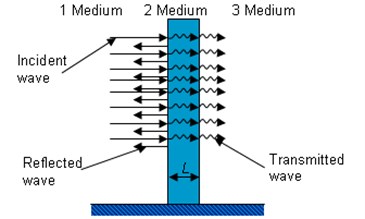
The sound transmission loss expresses the power transmission coefficient of the sound in decibel units:
where is the wave number in the th medium, is the thickness of the obstacle, , , are the characteristic impedances of the 1st, 2nd and 3rd media respectively. Secondly, these values of sound pressure on the boundary of the second and third mediums are used to excite and calculate the sound pressure in the acoustic medium once again. Eventually, the values of sound pressure calculated in the first and second stages are summarised using the principle of superposition, and the complete acoustic field in the closed spaces separated by the wall is calculated taking into account the loss of sound energy when the sound wave passes through the wall. In order to automate the calculations using the methodology, the macro file was created. It made the calculations much faster. To check the adequacy of the model created on the basis of FEM, a theoretical experiment was carried out. The theoretical experiment was based on the test of the propagation of sound from the source located in the closed space through the wall dividing the adjacent closed spaces. The results obtained by means of the FE model were compared to the results received using analytical model. The sound source was modelled as the source of sound propagating through the air, where the harmonic excitation frequency ranges from 30 Hz to 500 Hz. The calculations were carried out with the wall thickness of 200 mm and 250 mm. The sound pressure in the adjacent space was measured near the centre of the wall at the height of 1.5 m and at the distance of 0.5 m from it. FEM was applied to create the acoustic field model in the closed space. The obtained results of the theoretical calculation are provided below.
Fig. 2FE model of closed spaces separated by the wall
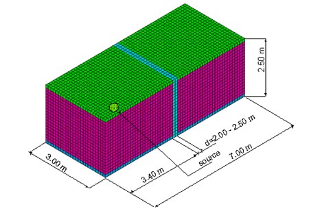
Fig. 3Sound pressure level in the adjacent room with regard to excitation frequency by using analytical and FEM model when the wall thickness is 25 mm
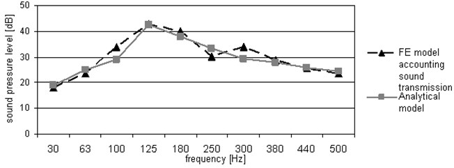
The comparison of the results of the theoretical experiment obtained by means of FE and analytical models shows a sufficiently high congruence. Such a congruence of results obtained can be observed over the entire frequency range from 30 Hz to 500 Hz. By means of the FE model designed in such a way, it will be possible to model the acoustic field in the closed space, taking into account sound wave reflection, diffraction in the event of obstacle and wave propagation through the obstacle.
3. Experimental test
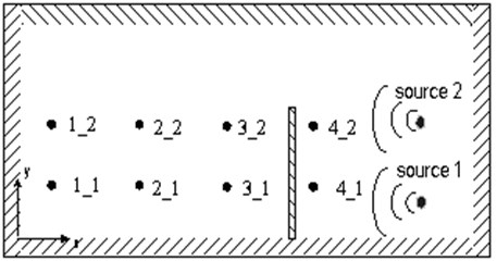
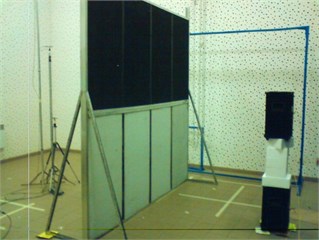
In order to check the adequacy of the theoretical model and its potential to be applied in the design of noise reduction systems in real conditions, i.e., with several noise sources present at a time, the experiment was carried out, and its results were compared with the theoretical ones. To that end, the FE model with a real closed space and a partition located in it was set up. In the model, the reflection of a sound wave, the diffraction under the conditions of the partition and its propagation through it were evaluated on the basis of the afore-discussed methodology. In order to imitate the experimental test, the initial data were selected accordingly: the value of sound pressure generated by sound source, its frequency, absorption coefficients of room’s planes and partition, etc. The acoustic partition (acoustic screen) was used in the experimental test. During the experiment the values of sound pressure were measured in front of and behind the acoustic partition in certain points. The principal scheme and general view of experimental measurement of sound pressure is shown in Fig. 4.
Fig. 4a) principal scheme, b) general view of sound pressure measurement
a)
b)
The marking of points shown in this scheme means the coordinates of microphone positions for example, the point marked as 1_2, has coordinate of 1 m and coordinate – 2 m; point 4_1 has coordinate of 4 m and coordinate of 1 m, etc. The coordinates of the first sound source shown in Fig. 4 are 5 m, – 0.25 m; the coordinate of the second sound source is 5 m, – 1.2 m.
When the analysis of sound propagation in the testing laboratory and its interaction with obstacles was done, the aforementioned method on the basis of FEM was used together with the harmonic analysis, during which the harmonic excitation at certain values of sound pressure in the analyzed frequencies was performed. Also, the values of sound pressure in different points presented in Fig. 4 were calculated by means of the analytical method, which is explained in greater detail in the [19]. The acoustic field in the testing laboratory was created using two loudspeakers. The values of sound pressure in different points of the testing laboratory in front of and behind the partition were measured using the device Investigator 2260 and the analyzer of vibrations and noise PULSE 3560 [20]. The results of the analytical model, experimental test and FE model received are presented below.
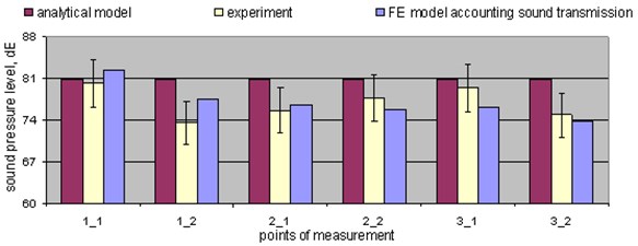
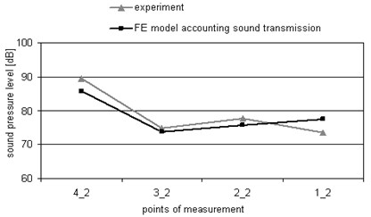
The comparison of the results of the experiment, FE and analytical models, where the experiment and the theoretical calculations were carried out in the closed space without a partition (Fig. 5), shows that the values of sound pressure calculated in different points by means of the FE model are more accurate than those obtained by means of the analytical method, i.e., as illustrated by Fig. 5, the values of sound pressure level obtained by means of the FE model do not exceed a 5 % error in 5 out of 6 measurement points compared to the values obtained by way of experiment. In contrast, the values of the level of sound pressure calculated by means of the analytical method do not exceed a 5 % error in 4 out of 6 measurement points. The results obtained with the measurements and calculations carried out in the closed space with a partition (Fig. 6) show that the values of sound pressure level calculated in all measurement points by means of the FE model do not exceed a 5 % error compared to those obtained by way of experiment, while in the case of the analytical method the values do not exceed a 5 % error in 3 out of 6 points only.
Fig. 5Values of sound pressure in different points in the testing laboratory when the excitation of 1000 and 2000 Hz is used at the same time. The measured experimental results are given with ±5 % (I) error bars (the arrangement of measurement points is shown in Fig. 4)
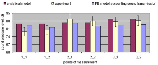
Fig. 6Values of sound pressure in different points in the testing laboratory with an obstacle in place when the excitation of 1000 and 2000 Hz is used at the same time. The measured experimental results are given with ±5 % (I) error bars
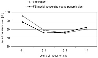
When the values of sound pressure level are compared separately at the height of one and two meters (Fig. 7(a, b)), the area of the so called partition’s “shadow” (the place behind the partition) is clearly seen, where the values of sound pressure are significantly lower than those in front of the partition. The dependencies received during the experiment confirm this fact. Thus, it is possible to state that the acoustic field created in the closed space under analysis is direct. When the values of sound pressure level are compared at the measurement points 3_1 and 3_2, located immediately behind the partition at the height of one and two meters, it is seen that the level of sound pressure at point 3_1 is higher by several decibels compared to point 3_2. It could be explained by the direction of sound emitted by the sources, i.e., the point at the height of one meter gets into the sound front emitted by the sources, and the waves that have passed through the obstacle and that have passed by it are summarized.
Fig. 7Levels of sound pressure were measured in different points when the excitation of 1000 and 2000 Hz is used at the same time: a) at the height of one meter; b) at the height of two meter
a)
b)
4. Conclusions
In this work, the model of acoustic field which takes into account the excitation of several sources, sound propagation in the closed space and its full interaction with obstacles (specially sound transmission through the obstacle, which is very important when the direct sound field is predominant if compared to the reflected field) in the real conditions on the basis of FEM is created.
The experiment revealed that the FE model allow to predict the values of the acoustic field’s parameters in the analysed point of the real object more accurate than the existing analytical methods.
The test of the adequacy of the theoretical model showed that it reproduces real fields adequately and it can be used for designing mobile and controlled systems of noise reduction.
References
-
Shuangli L., Hong N., Caijun X., Xin X. Aeroacoustic testing of the landing gear components. Journal of Vibroengineering, Vol. 14, Issue 1, 2012, p. 205-215.
-
Caijun X., Guang Z., Wei T., Shuangli L. Aeroacoustic noise reduction design of a landing gear structure based on wind tunnel experiment and simulation. Journal of Vibroengineering, Vol. 14, Issue 4, 2012, p. 1591-1600.
-
Ciskowski R. D., Brebbia C. A. Boundary Element Methods in Acoustics. Elseiver Applied Science, New York, 1991.
-
Filippi P., Habault D., Lefevre J. P., Bergassoli A. Acoustics, Basic Physics, Theory and Methods. Academic Press, New York, 1999.
-
Kludszuweit A. Time iterative boundary element method TIBEM – a new numerical method of four-dimensional system analysis for the calculation of the spatial impulse response. Acustica, Vol. 75, 1991, p. 17-27, (in German).
-
Kopuz S., Lalor N. Analysis of interior acoustic fields using the finite element method and the boundary element method. Applied Acoustic, Vol. 45, 1995, p. 193-210.
-
Yokota T., Sakamoto S., Tachibana H. Sound field simulation method by combining finite difference time domain calculation and multi-channel reproduction technique. Acoust. Sci. & Tech., Vol. 25, Issue 1, 2004, p. 15--3.
-
Yokota T., Sakamoto S., Tachibana H. Visualization of sound propagation and scattering in rooms. Acoust. Sci. & Tech., Vol. 23, Issue 1, 2002, p. 40-46.
-
Matsumoto G., Fujiwara K., Omoto A. Directivity of the sound radiated from a factory building. Acoust. Sci. & Tech., Vol. 22, Issue 6, 2001, p. 434-436.
-
Randall F. B. Industrial Noise Control and Acoustics. Marcel Dekker, New York, 2001.
-
Beranek L. L. Acoustics. Acoustical Society of America, New York, 1996.
-
Wright M. C. Lecture Notes on the Mathematics of the Acoustics. Imperial College Press, London, 2005.
-
Everstine G. C. Finite element formulation of structural acoustics problems. Comp. & Structures, Vol. 65, 1997, p. 307-321.
-
Salin M. B., Sokov E. M., Suvorov A. S. Calculation of the acoustic bistatic target strength of objects with complicated internal structure using FEM. Proceedings of the 10-th European Conference on Underwater Acoustics (ECUA), Istanbul, 2010, p. 1117-1124.
-
Daniel R. R. The Science and Applications of Acoustics. Second Edition, Springer, New York, 2006.
-
Von Estorff O. Modern Numerical Methods to Solve Real Life Acoustics Problems. Proceedings of the 6-th Forum Acusticum, Aalborg, 2011, p. 17-18.
-
Lohrenscheit T., Kletschkowski T., Sachau D. Vibro-Acoustic Finite Element Analysis of a Full-Scale Aircraft Mock-up. Proceedings of the 6-th Forum Acusticum, Aalborg, 2011, p. 167-172.
-
Mikalauskas R., Volkovas V. Modeling of sound propagation in the closed space and its interaction with obstacles. Mechanika, Vol. 6, Issue 80, 2009, p. 42-47.
-
Randall F. B. Industrial Noise Control and Acoustics. Marcel Dekker Inc., New York, 2003.
-
Volkovas V., Slavickas E. S., Gulbinas R. J. The Investigation of Effectiveness of Acoustical Isolation of Noise Sources. Proceedings of the 14-th international conference Mechanika, Kaunas, 2009, p. 445-448.
About this article
