Abstract
The deformation detection of large machinery is usually achieved using three-dimensional displacement measurement. Binocular stereo vision measurement technology, as a commonly used digital image correlation method, has received widespread attention in the academic community. Binocular stereo vision achieves the goal of three-dimensional displacement measurement by simulating the working mode of the human eyes, but the measurement is easily affected by light refraction. Based on this, the study introduces particle swarm optimization algorithm for target displacement measurement on Canon imaging dataset, and introduces backpropagation neural network for mutation processing of particles in particle swarm algorithm to generate fusion algorithm. It combines the four coordinate systems of world, pixel, physics, and camera to establish connections. Taking into account environmental factors and lens errors, the camera parameters and deformation coefficients were revised by shooting a black and white checkerboard. Finally, the study first conducted error analysis on binocular stereo vision technology in three dimensions, and the relative error remained stable at 1 % within about 60 seconds. At the same time, three algorithms, including the spotted hyena algorithm, were introduced to conduct performance comparison experiments using particle swarm optimization and backpropagation network algorithms. The experiment shows that the three-dimensional error of the fusion algorithm gradually stabilizes within the range of [–0.5 %, 0.5 %] over time, while the two-dimensional error generally hovers around 0 value. Its performance is significantly superior to other algorithms, so the binocular stereo vision of this fusion algorithm can achieve good measurement results.
1. Introduction
In the modern industrial society, with the rapid development of Digital Image Correlation Method (DIC) based on Binocular Vision Ranging technology (BVR), users can remotely measure the displacement of large civil elements, and then judge the safety of the structure through its deformation [1, 2]. To accurately calculate the displacement of the mechanical structure, BVR sets up two cameras, which are placed in a triangular shape with the target to be measured. By continuously changing the position of the target through an electronically controlled 3D displacement table, the camera can collect a series of data and calculate the displacement of the target. However, the working principle of the camera is small aperture imaging, and the propagation of the light path is not only limited by environmental changes, but also causes light displacement when entering and exiting the lens. The error of the constructed binocular 3D ranging model is too large, which does not meet the application requirements [3]. In recent years, Particle Swarm Optimization Algorithm (PSO) has attracted the attention of many scholars due to its advantages such as wide global search range [4]. PSO is a biomimetic bird swarm with the ability to capture images of moving targets. But PSO has weak local search ability during iteration, and its particles are prone to falling into local optima, resulting in significant errors in the results. For improving this condition, this study is based on the powerful learning ability of BP neural networks. By adjusting the weight threshold in the network, a fusion algorithm with strong local search ability, BP Neural Network Fusion PSO (BPSO) is generated. However, the traditional BP neural network cannot deal with the complex nonlinear model with unknown conditions, which will eventually lead to overfitting and accuracy reduction. PSO algorithm, which can make it change from disorder to order, can deal with this defect well. Meanwhile, PSO algorithm can also use the optimal initial weight threshold of BP neural network to realize the global optimization process. The two complement each other and finally achieve high-precision prediction results. The mutated particles have dynamic learning ability and can jump out of local optima. The research is mainly divided into four chapters. The first part mainly introduces the working principle and measurement principle of binocular stereo vision cameras. The second part conducted on previous relevant studies a literature review. The third part introduces the factors that affect ranging technology and the construction of a dual camera ranging prediction model for DIC. The fourth part analyzes and compares the performance of this optimization model with traditional models. The last part of the simulation experiment was conducted on the Canon imaging dataset, pointing out the shortcomings that still exist in the research. This study aims to improve the problem of long working hours and weak learning ability in PSO, which has profound significance for hazard prediction in practical engineering.
2. Related works
The deformation of materials is very common, and scholars in various fields are also committed to the optimization of material stability. Jena et al. [5] believed that aluminum metal matrix composite is an important structural material with excellent properties such as low density and high specific strength. Therefore, scholars use it for crack analysis and introduce finite element method for crack failure analysis, and the results show that the crack analysis results of this material are excellent. Bal et al. [6] realized that structural damage is inevitable in engineering materials, so it is very necessary to study the fracture mechanical properties of materials, and damage diagnosis is also a key module. The study analyzed the dynamic behavior of epoxy glass fiber composite beams through a one-dimensional model based on the coupling effect of bending and torsion, and introduced finite element analysis. By calculating the relative natural frequency and other data, the effect of crack depth and location on the dynamic characteristics of the beam was studied. Parida and Jena [7] studied the stress component, static deflection and natural frequency of materials, and compared the hypothesized theoretical results with the results of first-order shear deformation theory and finite element analysis, respectively, to compare and optimize the effects of different filling materials.
In large-scale civil engineering, the deformation measurement of structure is often used for safety monitoring. The safety and reliability of the previous contact measurement are low, so the non-contact 3D displacement measurement technology has been gradually developed. At the same time, due to the continuous iteration of the camera industry, the new digital image correlation method technology has also been paid attention to, and is often used in the measurement of position change in engineering. The three-dimensional displacement analysis of images, as an important branch of position change technology, plays a very important role in construction hazard prediction, casting life prediction, and other aspects. Li and Zhang [8] introduced binocular ranging technology to study the movement displacement of athletes through the measurement method of wireless sensing parameters. To discuss the connection of mechanical parameters, the movement patterns of athletes are analyzed, providing theoretical guidance for their physical training. They developed a non-contact displacement measurement system that uses templates to extract the image coordinates of measurement points, and restores the spatial coordinates of measurement points through Euclidean three-dimensional reconstruction. In the vibration testing of cantilever beams, a binocular image displacement measurement system was utilized to assess the displacement of the cantilever beam, and the high accuracy of the system was finally verified. Genovese [9] proposed a comprehensive DIC method to achieve mobile phones with full field information of large deformation biological surfaces. This study expands the view covers of traditional binocular stereo DIC systems to 36×320. At the same time, it uses a new iterative image deformation scheme and a feature based robust algorithm to calculate the total disparity between images. Next, by using a hybrid local DIC method, the iterative strength interpolation correlation has been refined. Finally, under replicated physiological loads, they conducted full field DIC shape and deformation measurements on pig eyes tested in vitro. The shape and material complexity of this model are almost unlimited. Guo et al. [10] proposed an extended DSO binocular stereo positioning algorithm based on the Direct Sparse Method (DSO). This algorithm has strong robustness and can expand the sensors of panoramic vision, which can directly obtain panoramic depth images around vehicles, and its robustness is far superior to other ordinary visual odometers. It will have broad application prospects. Li and Zhang [11] proposed an anisotropic distance measurement method for subway travel to study the residential convenience index of buildings in the urban area of Beijing. The spatial distribution results of residential buildings at all levels in the city indicate that considering subway travel, the convenience indicators of residential buildings at all levels are more reasonable.
Wang and Hu [12] proposed an improved feature stereo matching algorithm, which first preprocesses and extracts features from the left and right images, and uses filtering to obtain matching points. Set the obtained matching points as seed points, establish a continuous search space based on the human eye disparity criterion, and then achieve bidirectional regional growth through matching strategies. The study conducted simulation experiments using the Middlebury dataset and found that the algorithm has high-precision disparity and can improve the matching effect in deep discontinuous areas. Moreover, it has great robustness and can suppress the impact of brightness differences and noise. Fadiji et al. [13] determined the compressive load of corrugated cardboard packaging with displacement through three-dimensional digital images, and the strain field was derived from the displacement field. They measured the bending data of corrugated cardboard based on the results obtained from the displacement field, and also observed that the displacement was uneven, with the horizontal axis being smaller than the displacement fields in the vertical and vertical axes. In the experiment, the change in strain increases with the increase of load, and they speculate that it is a precursor to the failure of this material. This technology is effective in handling the variables related to surface displacement and strain field in corrugated cardboard packaging of horticultural products. Their experiments have shown that it has the potential to improve the packaging of fresh agricultural products. Xie et al. [14] proposed a low-cost panoramic DIC system. It includes two binocular stereo DIC systems and one flat mirror, which can test full surface shape reconstruction and deformation. The back surface of the substance can directly capture the sample, and the stereo DIC system of the front surface is used for reconstruction. Draw 6 speckle patterns on the reflector to convert the surface into common coordinates. Their proposed technology can provide accurate full surface state and displacement data, with advantages such as low cost and high robustness.
The application of binocular stereo vision technology in three-dimensional displacement measurement is very extensive, but there is not enough research on improving the integration of relevant algorithms. This study groundbreaking combines backpropagation neural networks with PSO, taking into account the impact of environmental factors and lens thickness, to achieve better binocular stereo vision measurement results.
3. Image 3D displacement detection based on binocular stereo vision
The DIC combines the visual field with image measurement, utilizing the deformation distance of the target point to obtain displacement data of the image. Binocular stereo vision is a method that utilizes the principle of DIC to achieve three-dimensional displacement detection of images [15].
3.1. The workflow and model establishment of BVR measurement technology
The eyes recognize three-dimensional objects through a triangular area formed by binocular parallax and the target, and binocular vision measurement technology is designed based on this. This technology utilizes two cameras to simulate the eyes, placing them at different positions and angles, and capturing the target point at the same time. Finally, the collected images will be calculated and analyzed to acquire the 3D data of the target point. The workflow of BVR measurement technology roughly includes image acquisition, camera calibration, feature extraction and matching, and 3D reconstruction [16]. The foundation for achieving three-dimensional measurement is the correct use of cameras to collect data. The camera imaging principle can be roughly divided into two parts: coordinate conversion and model establishment. The pixel coordinates and physical coordinates of the known image belong to the coordinate system (CS) of two-dimensional space, where represents the pixel CS, and the unit is Pixel; - is the physical CS, expressed in millimeters. The origin of the pixel CS is located in the upper left corner of the image, while the origin of the physical CS locates at the center point of the image. Set the pixel value coordinate of center point to , and represent the physical axis dimensions of each pixel as and . The conversion relationship between the two coordinates is Eq. (1):
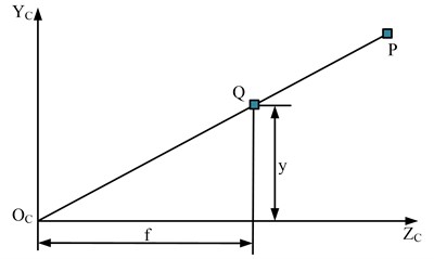
In the three-dimensional camera CS -, represents the optical center of the lens; represents the focal length of the camera. The world CS - can represent the spatial relationship between the camera and the target. The camera coordinate of the target position and the world coordinate need to be further converted and calculated, as shown in Eq. (2):
where, is rotation matrix; represents the translation vector; is the external parameter matrix; represents the origin of the world coordinate system in the camera coordinate system. The two-dimensional coordinates of the image are transformed through the camera CS and ultimately mapped to the three-dimensional world CS. In theory, the entire process is linear, usually completed using a pinhole projection model, as shown in Fig. 1.
When a beam of light passes through the pinhole, a projection image is formed on the back of the pinhole. All coordinates in the pinhole projection model are linear transformation, which is an ideal model, which can map three dimensions to two dimensions. At the same time, due to the existence of the lens on the camera lens, the process of projecting light onto the imaging plane will be distorted. Therefore, it is necessary to combine the distortion model to describe the whole projection process. Finally, the external three-dimensional points are projected onto the internal imaging plane of the camera to form the internal parameters of the camera. However, in practical applications, due to the lens distortion problem that often accompanies camera shooting, the pixel value coordinates obtained are not the same as the actual coordinate data.
Fig. 1Linear pinhole projection model
Based on this, a nonlinear model considering the influence of distortion is introduced in the study, see Eq. (3):
where, represents the theoretical pixel coordinates; is the actual measured pixel coordinates; represents the magnitude of distortion in different directions. When disorderly refraction occurs during light irradiation, distortion of the lens occurs. Distortion could be separated into radial and tangential directions according to different directions, and the reasons for the two types of distortion are lens shape and lens assembly. This is also the reason for transforming the theoretical linear transformation process into an actual nonlinear process, and this problem will increase the complexity of modeling. When there are too many nonlinear parameters, the stability and accuracy of the calculation results will decrease [10]. Therefore, research often only takes radial distortion as the overall description, see Eq. (4):
where, represents the distortion value, and usually only lower order coefficients are considered. Radial distortion can be divided into barrel distortion and pillow distortion. The former means that the pixels in the center part of the image are too small, while the pixels in the edge part are too large, resulting in the straight line bending to the edge of the image; The latter is the opposite of the former, that is, the pixels in the center part of the image are larger, and the pixels in the edge part are smaller, making the line bend toward the center of the image. The radial distortion parameter is mainly used to correct the distortion in the image taken by the camera. When correcting the image, it is necessary to measure the distortion parameter value of the camera, and then correct the image according to the measurement results. Zhang’s calibration method is used to measure the distortion function, as shown in Eq. (5):
where, and respectively represent ideal pixel coordinates and distorted pixel coordinates; and respectively represent ideal normalized coordinates and distorted normalized coordinates. The maximum likelihood theory is used to solve the optimal solution, and LM algorithm is introduced to calculate the minimum parameter value, as shown in Eq. (6):
The above Eq. (6) represents points in images. The structure of the binocular vision measurement model includes dual cameras and target points, as shown in Fig. 2.
Fig. 2Binocular vision measurement model
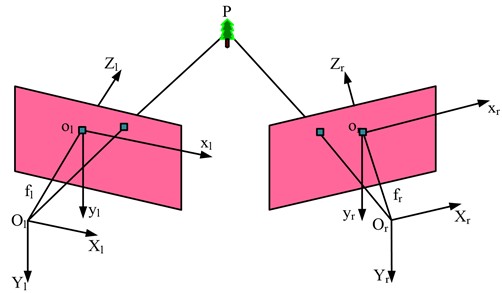
In Fig. 2, and represent the left and right cameras, respectively; The CSs of the camera and image are represented as - and - respectively; is the effective focal length; represents the target point. The three-dimensional coordinate values of the target point can be obtained by combining the coordinates measured by the cameras on both sides. The measurement model usually includes polar constraints that can obtain the relationship between the coordinates of the two cameras on both sides, as shown in Fig. 3.
Fig. 3Schematic diagram of camera polar constraint line
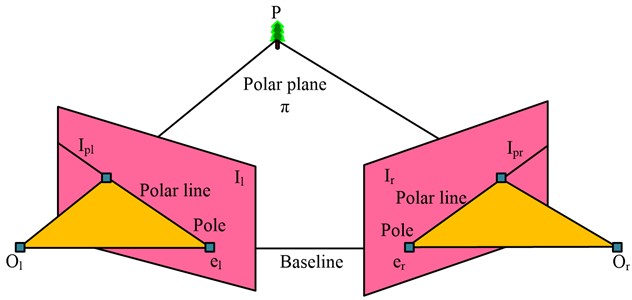
In Fig. 3, and represent the imaging planes of the left and right cameras, respectively; and represent the imaging points of target point in the camera; The connecting line of the optical center is the baseline; The connecting lines between the optical centers on both sides and the target point form the polar plane. That intersection of the baseline and the imaging surfaces on both sides is the pole, represented by and ; The intersection line between the polar plane and the imaging surfaces on both sides is the polar line, represented by and . The polar constraint indicates that when either imaging point is located on the imaging surface in its corresponding direction, the other imaging point must be located on the polar line of the imaging surface in its corresponding direction. The ideal imaging point coordinates for both cameras are and , respectively, and the relationship between the two can be expressed by Eq. (7):
where, represents the basic matrix, which is related to the inter and outer parameters of the camera, as Eq. (8):
where, represents the translation vector transformation; respectively represent the internal parameter matrix of the left and right cameras. Based on the imaging point coordinates of the cameras on both sides, the three-dimensional coordinate values of the target point can be calculated. Before the camera captures images, it should first perform camera calibration and record the internal and external parameters of the camera. It includes five parameters: scale factor , focal length , distortion factor , rotation matrix and translation vector . The parameters obtained from calibration are the key to achieving accurate measurement, so this step is the most fundamental and important step in the entire measurement process. The camera calibration process is Fig. 4.
Fig. 4Camera calibration process
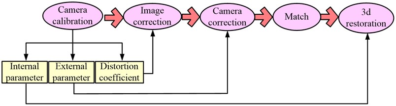
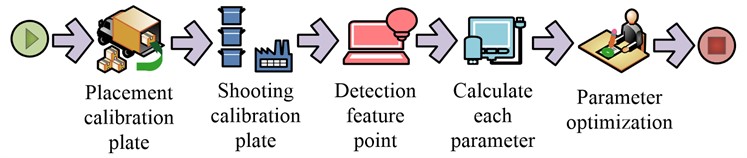
Camera calibration is the process of estimating the parameters of the camera model, and obtaining the parameters of the internal geometry of the process by describing the image. Accurate camera calibration is essential for a variety of applications, such as the correlation of images from multiple cameras, as well as the elimination of geometric distortions due to imperfect lenses, or the accurate measurement of real-world geometric properties (position, distance, area, straightness, etc.) data. Therefore, its essence is to construct an imaging geometric model from the parameters obtained by calibration, and to construct a three-dimensional scene from this. Camera calibration can be roughly segmented into classic calibration methods and self calibration methods. The accuracy of the classical method is higher, but the premise is that the accuracy of the calibration object itself is high, and the self calibration method usually cannot meet basic needs. The research uses checkerboard calibration, which performs better in terms of accuracy and generalization, and the operation is not complex, solving the problem of dependence on the accuracy of the calibration object in traditional calibration [17]. The chessboard calibration method, also known as the Zhang Zhengyou calibration method, is a method that only requires a single black and white chessboard to achieve the required calibration effect. It has excellent performance in terms of practicality and accuracy. The workflow is Fig. 5.
In Fig. 5, it is necessary to first place the calibration board on a certain plane, take images of the calibration board at different angles, extract image feature points, and then calculate the camera’s internal and external parameters and distortion coefficient, and finally optimize the parameters. Known points are represented as and in the 3D world CS and the 2D pixel CS, respectively. According to the expressions of each parameter, the relationship between the two can be simplified to the equation shown in Eq. (9):
where, and are orthogonal matrices; is the product of two orthogonal matrices; represents the non-vertical factor, approximately 0; represents an internal parameter matrix; is a matrix vector. To achieve the calculation of three-dimensional and two-dimensional coordinates, the calibration board is set to be located at position in the world CS, and its world coordinate is . Setting the homography matrix requires 8 parameters to solve, where the world and pixel coordinates are known. The matrix is obtained by combining the internal and external parameter matrices of the camera.
Fig. 5Checkerboard calibration process
4. Design of image measurement model introducing BP and PSO
To avoid the impact of various environments and self errors on the measurement results during actual measurement, a model integrating BP neural network and PSO is introduced to improve it. BP is adept at handling nonlinear structures, with advantages such as high accuracy and ease of operation. It consists of three layers of input, hidden, and output. After the neurons in the input layer reach the threshold, the forward signal propagation and reverse inter system jump are triggered, and the hidden layer is activated. After the status update, the intermediates of the hidden layer are obtained and compared with the preset values in the output layer. When the difference between the two is lower than the minimum error requirement, the result is output and the iteration ends. As the number of hidden layers increases, the experimental error decreases, and in practice, it varies according to the complexity of the input values. The computational speed of a network is related to the number of hidden layer nodes. If there are too many nodes, it is easy to fall into local optima, and if there are too few nodes, it will prolong the iteration time [18]. This study introduces Formula (10) to optimize the number of hidden layer nodes:
where, the node numbers in the three layers are denoted as and is the constant in the interval [0, 10]. The BP neural network uses additional momentum to update the threshold, as shown in Eq. (11):
where, represents the weight values at different times; is the learning rate. Traditional BP neural networks are only suitable for linear fitting data, but actual experiments may involve nonlinear models. So dynamic learning is introduced to improve the BP neural network, using the method of adjusting negative gradients to update the threshold, as shown in Eq. (12):
where, represents learning efficiency, and the region time is denoted as . The meaning of is the time required to achieve the highest learning efficiency , and the minimum learning efficiency during this period is represented by . PSO is a biomimetic bird swarm, where the particles in PSO are compared to birds, and the bird that finds food is called the optimal solution. In this algorithm, the particle is compared to a bird, that is, it has three characteristic values of velocity, position and fitness value. Each particle is a problem to be optimized in the solution space, and its movement characteristics are related to the speed, and the dynamic fluctuation of the speed is related to the movement experience between the particles. The particle recalculates the fitness function at the same time as the position is updated, and the data is used as the basis for the update [19]. The remaining particles will move towards the optimal solution, which is called iteration. The iterative process is Eq. (13):
where, the inertia weight is denoted as , the particle velocity is selected as , and the range of , values is non negative, which is called the learning factor. , represent the global optimal position and the local optimal position, respectively. In the early stages of PSO iteration, a slightly larger value of can expand the global search range; At the end of the iteration, a smaller value is required, which is suitable for local search. The formula for the value of is Eq. (14) [20]:
where, the initial and ending values are denoted as , , and the number of iterations is represented by . The maximum number of iterations for PSO is . However, in practical application, the inertia weight in the early stage is prone to a cliff like drop, resulting in a small in the later stage and prolonging the algorithm’s working time [21]. To solve this problem, the sigmond function was introduced to adjust Eq. (14) and obtain Eq. (15):
where, the value of , varies with the operation of PSO. Compared to traditional algorithms, PSO has the advantages of high convergence speed and wide adaptability, but it is prone to falling into local optima. The study utilizes the variability of BP neural networks to fuse them with PSO, enabling PSO particles to have mutation ability and undergo random initialization to jump out of local optima. The mutation process of PSO is Eq. (16):
where, represents the diagonal length value of the space, and the population size is denoted as . The meaning of is the coordinates of particles, and the mean of all particle coordinates is represented by . The mutation PSO algorithm has the ability to control particle spacing. When the spacing is less than the inertia weight, the algorithm is already in local optimization. At this point, particles with poor optimization results will undergo mutation, and the mutation probability is as follows Eq. (17):
where, represents the Gaussian constant, with a value range of . The fitting accuracy and global search speed of the composite algorithm BPSO can be significantly improved, as shown in Fig. 6.
Fig. 6Fusion algorithm of mutated PSO and improved BP neural network
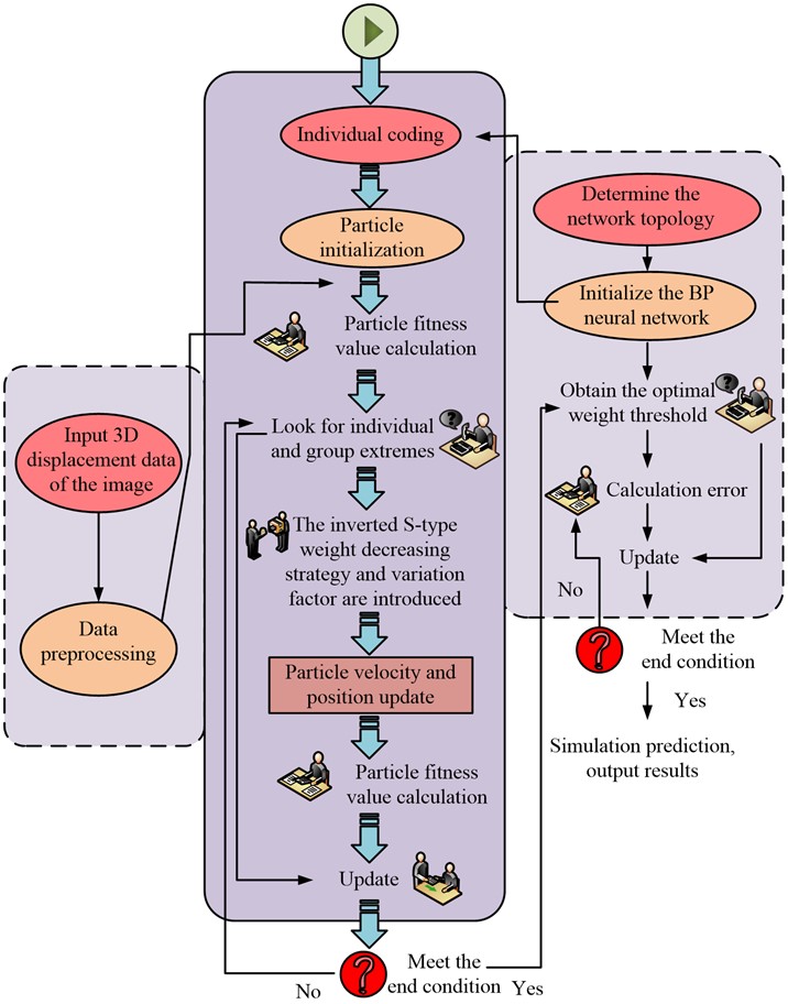
In Fig. 6, the iteration of BPSO first requires measuring the displacement values of the image on the three axes as input to the algorithm. Then it is pretreated, and the fitness value of particles is calculated as a candidate group for individual extreme value and group extreme value. Determining the network structure again, to initialize the BP and obtain the optimal threshold. Finally, the particle positions and velocities updated by the mutation factor together gathered to determine whether the algorithm termination conditions are met [22]. If the weight reaches the threshold, the algorithm terminates and outputs calibrated data; If the weight value does not reach the threshold, the error will be recalculated. Among them, the value of neuron connection between different layers in BP network is the weight value, and the whole operation is divided into forward propagation and reverse feedback. In the former, the data is passed from the input layer to the hidden layer for processing, and then the output value is compared with the theoretical value by the output layer. If the error exceeds the allowable range, it should be re-optimized and corrected through reverse transmission. Therefore, the final output value obtained by BP neural network can be used as the basis for individual coding of PSO algorithm, that is, initialization of particle data information, and the best initial cluster can be selected on this basis.
4.1. Performance of a binocular vision measurement model incorporating BP and PSO
A three-dimensional electrically controlled displacement experimental platform was selected for the study. The left and right cameras were built into a triangular pattern with the electrically controlled three-dimensional displacement platform, and connected to a computer, as Fig. 7.
Fig. 7Experimental equipment diagram
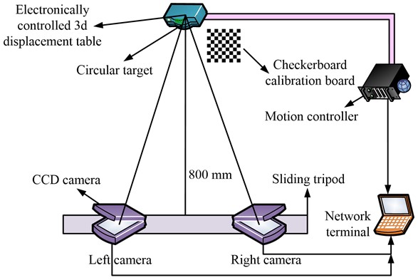
As Fig. 7, first, the target images taken by the left and right cameras will be input into the computer, and then the motion controller will move the target irregularly. The electronic 3D displacement table will record this process, and finally the tripod will slide and load data to obtain the output result of the guide rail. The models of each instrument are displayed in Table 1.
In addition, the study sets the input and output of BP network as three-dimensional, the number of nodes in the input and output layers is 3, and the number of nodes in the two hidden layers is 15 and 14 respectively, so the weight and threshold of the network are 297 and 32, respectively. The individual encoding length of the PSO algorithm is 329.
Table 1Models of experimental instruments
Instrument | Parameter |
Camera | SONY HDR-PJ675 |
Optical lens size | 36 mm |
Camera pixel | 9.2 million |
Camera frame frequency | 60 Hz |
Electronically controlled shift station | Zhuo Li Han Guang (TMC-USB) |
Round target outside/inside diameter | 60/30 mm |
Calibration plate | 12×9 |
Calibration panel size | 10×10 mm |
Base distance | 20 mm |
Camera angle | 20° |
Object distance | 800 mm |
Distance of the camera from the ground | 1200 mm |
Data set | Canon |
4.2. BVR measurement system performance
This study establishes the above experimental environment to achieve accuracy detection of BVR measurement models. Before the experiment, it is necessary to initialize the instrument and adjust the three dimensional directions of the electronic displacement table to the 10 mm scale value at a speed of 0.1 mm/s. The sampling frequency of the dual cameras is adjusted to 1 HZ, and the number of frames collected by the circular target is 100. The absolute error and relative error results of the binocular vision measurement model obtained in the experiment are Fig. 8.
Fig. 8Error results of binocular vision measurement model
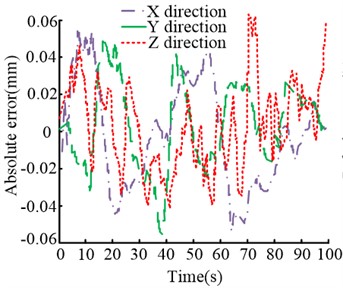
a) The absolute error in each direction
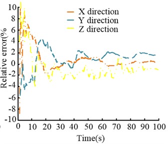
b) The relative error in each direction
In Fig. 8(a), the absolute error of the binocular vision measurement system in three directions is within the range of (–0.06, 0.08), its stability is relatively high, and the fluctuation gradually decreases with time. The trend of change in that three directions is roughly the same, with the error reaching a peak of 0.071 mm in the direction around the 70th second. In Fig. 8(b), the relative error changes of the system in three directions are gradually restored to stability over time. The average relative error in the direction is the smallest, and the fluctuation is also the lowest. Although the initial relative error in both the and directions reached over 9 %, they both fell into a relatively lower error range within 20 seconds. Finally, the relative errors in all three directions were basically stable within 1 %. The initial error is relatively large, and the key lies in the small value of the initial data itself. To sum up, the relative error and absolute error of the binocular vision measurement system are within the reliable range.
4.3. Performance of binocular vision measurement system introducing BPSO model
The principle of image displacement measurement is to use the deformation position of the target point on the speckle image to obtain the offset. To further verify the performance impact of introducing BPSO on binocular vision measurement systems, the study first conducted experiments on its image computing ability. Fig. 9 is the results.
Fig. 9Ability of left and right cameras to capture images
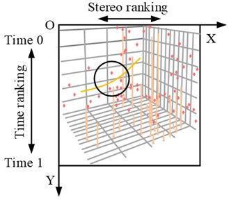
a) Left camera target
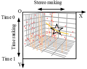
b) Right camera target
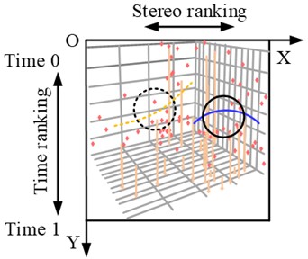
c) Left camera calibration
d) Right camera calibration
Fig. 9 shows the labeling process of dual cameras for target fixed points. Although there are a large number of unrelated interference points around the target point, BPSO can also successfully locate the position of the target point. So there is no need for manual speckle, further realizing the automated speckle process and greatly improving the system's work efficiency. After a series of initialization operations, the study used intersection method to label images. To further validate the performance of BPSO, the traditional Spotted Hyena algorithm (SH), Long term and Short term Memory network (LSTM), and individual PSO algorithms were introduced for comparative analysis. Fig. 10 shows the results.
In Fig. 10, when the algorithm runs for about 70 seconds, the error values of BPSO and PSO remain stable, with fluctuations gradually decreasing. The total error fluctuates around –0.5 % and 0.5 %, respectively. However, the SH algorithm and LSTM have not stabilized, and the error fluctuation range of SH and LSTM is wider, with a maximum error value of over 0.9 %. Only comparing the total errors of the four algorithms cannot distinguish the optimal algorithm. Therefore, the study analyzed the two-dimensional coordinate axis errors of each of them and the error changes in the calibration experiment, and plotted the images as exhibited in Fig. 11.
Fig. 10Comparison of error performance of each algorithm
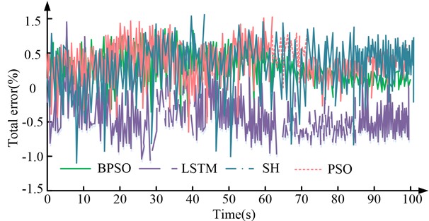
Fig. 11Comparison of two-dimensional errors and calibration errors of the algorithm
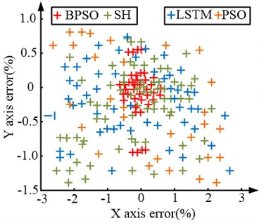
a) Two-dimensional axis error view
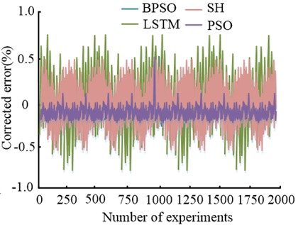
b) Calibration experiment error
From Fig. 11(a), the experimental results of the BPSO model are concentrated in the range of total error around 0, the error range of the -axis is within the range of [–1 %, 1 %], and the error range of the -axis is mostly distributed within the range of [–0.5 %, 0.5 %]. The error distribution of other algorithms is wide, and the parts with larger errors are sparsely distributed. The -axis error is approximately [–3 %, 3 %], while the -axis error is approximately [–1.5 %, 1.0 %]. By comparison, the performance of BPSO is far superior to other algorithms. In the 2000 error correction experiments of Figure 11(b), the LSTM had the largest error variation range, recorded as [–0.7 %, 0.6 %]; Next is the SH algorithm, which has a calibration experiment error range of [–0.5 %, 0.5 %]. The error range difference between PSO and BPSO is the smallest, between the range of [–0.13 %, –0.03 %]; The error curve of BPSO fluctuates between –0.02 % and 0.04 %, with the smallest fluctuation range. The above results verify that BPSO has the smallest error and relatively gentle fluctuations, which meets the requirements of DIC method for measuring object displacement. Therefore, the BVR measurement system incorporating BPSO has good image displacement measurement performance.
5. Conclusions
With the development of heavy industrial society, three-dimensional displacement detection of large construction machines is particularly important. This study utilizes a widely used BVR system for displacement measurement to detect whether the target object is deformed. To solve the error problem caused by light refraction and other factors, research has introduced BP neural network and PSO algorithm for improvement. Finally, a three-dimensional displacement measurement test bench was built and simulated using the Canon dataset. First of all, a separate error analysis was conducted for the BVR system: the absolute error of the system in the three-dimensional direction fluctuated within the range of [–0.06 mm, 0.08 mm], and the relative error stabilized at about 1 % in 60 s. Subsequently, experiments were conducted on the image computing ability of BPSO: in the presence of a large amount of interference information, the algorithm can still correctly recognize effective information. To further analyze the performance of BPSO, comparative experiments were conducted with three algorithms such as LSTM. In the three-dimensional dimension, after 70 seconds of three-dimensional running time, the error of BPSO basically fluctuated between –0.5 % and 0.5 %; The fluctuation of LSTM and SH has always been significant, and varies within the error range of –1 % to 1.5 %. In the calibration experiment error analysis, the error of BPSO is between 0.02 % and 0.04 %, and the error of LSTM is within the range of [–0.7 %, 0.6 %]. The above experiments indicate that the BVR system incorporating the BPSO algorithm has excellent performance and can achieve good 3D displacement measurement results.
References
-
H. Wang, G. Dou, H. Zhang, X. Zhu, and L. Song, “3D velocity field reconstruction of gas-liquid two-phase flow based on space-time multi-scale binocular-PIV technology,” Optoelectronics Letters, Vol. 18, No. 10, pp. 613–617, Oct. 2022, https://doi.org/10.1007/s11801-022-2007-8
-
Y. Zhang et al., “Accurate profile measurement method for industrial stereo-vision systems,” Sensor Review, Vol. 40, No. 4, pp. 445–453, Jun. 2020, https://doi.org/10.1108/sr-04-2019-0104
-
J. Yang and K. Bhattacharya, “Augmented lagrangian digital image correlation,” Experimental Mechanics, Vol. 59, No. 2, pp. 187–205, Feb. 2019, https://doi.org/10.1007/s11340-018-00457-0
-
A. F. A. Ghani, R. Jumaidin, M. S. F. Hussin, S. D. Malingam, and R. Ranom, “Digital image correlation (DIC) and finite element modelling (FEM) assessment on hybrid composite carbon glass fibre under tensile and flexural loading,” International Journal of Mechanical and Mechatronics Engineering, Vol. 20, No. 3, pp. 82–90, 2020.
-
P. C. Jena, D. R. Parhi, G. Pohit, and B. P. Samal, “Crack assessment by FEM of AMMC beam produced by modified stir casting method,” Materials Today: Proceedings, Vol. 2, No. 4-5, pp. 2267–2276, 2015, https://doi.org/10.1016/j.matpr.2015.07.263
-
B. B. Bal, S. P. Parida, and P. C. Jena, “Damage assessment of beam structure using dynamic parameters,” in Lecture Notes in Mechanical Engineering, Singapore: Springer Singapore, 2020, pp. 175–183, https://doi.org/10.1007/978-981-15-2696-1_17
-
S. P. Parida and P. C. Jena, “A simplified fifth order shear deformation theory applied to study the dynamic behavior of moderately thick composite plate,” in Applications of Computational Methods in Manufacturing and Product Design, Singapore: Springer Nature Singapore, 2022, pp. 73–86, https://doi.org/10.1007/978-981-19-0296-3_8
-
H. Li and B. Zhang, “Application of integrated binocular stereo vision measurement and wireless sensor system in athlete displacement test,” Alexandria Engineering Journal, Vol. 60, No. 5, pp. 4325–4335, Oct. 2021, https://doi.org/10.1016/j.aej.2021.02.033
-
K. Genovese, “An omnidirectional DIC system for dynamic strain measurement on soft biological tissues and organs,” Optics and Lasers in Engineering, Vol. 116, No. 5, pp. 6–18, May 2019, https://doi.org/10.1016/j.optlaseng.2018.12.006
-
X.-D. Guo et al., “Research on DSO vision positioning technology based on binocular stereo panoramic vision system,” Defence Technology, Vol. 18, No. 4, pp. 593–603, Apr. 2022, https://doi.org/10.1016/j.dt.2021.12.010
-
J. Li and S. Zhang, “Research on Beijing residential convenience index based on point of interest,” Journal of Computer-Aided Design and Computer Graphics, Vol. 33, No. 4, pp. 609–615, Apr. 2021, https://doi.org/10.3724/sp.j.1089.2021.18539
-
D. Wang and L. L. Hu, “Improved feature stereo matching method based on binocular vision,” Acta Electronica Sinica, Vol. 50, No. 1, pp. 157–166, 2022, https://doi.org/10.12263/dzxb.20200919
-
T. Fadiji, C. J. Coetzee, and U. L. Opara, “Evaluating the displacement field of paperboard packages subjected to compression loading using digital image correlation (DIC),” Food and Bioproducts Processing, Vol. 123, pp. 60–71, Sep. 2020, https://doi.org/10.1016/j.fbp.2020.06.008
-
R. Xie, B. Chen, and B. Pan, “Mirror-assisted multi-view high-speed digital image correlation for dual-surface dynamic deformation measurement,” Science China Technological Sciences, Vol. 66, No. 3, pp. 807–820, Mar. 2023, https://doi.org/10.1007/s11431-022-2136-1
-
Y. Li, Z. Cheng, C. Yang, M. Wei, and J. Wen, “Application of binocular stereo vision in radioactive source image reconstruction and multimodal imaging fusion,” IEEE Transactions on Nuclear Science, Vol. 67, No. 11, pp. 2454–2462, Nov. 2020, https://doi.org/10.1109/tns.2020.3022103
-
R. Wang et al., “Accuracy study of a binocular-stereo-vision-based navigation robot for minimally invasive interventional procedures,” World Journal of Clinical Cases, Vol. 8, No. 16, pp. 3440–3449, Aug. 2020, https://doi.org/10.12998/wjcc.v8.i16.3440
-
M. Unver, M. Olgun, and E. Ezgi Turkarslan, “Cosine and cotangent similarity measures based on Choquet integral for Spherical fuzzy sets and applications to pattern recognition,” Journal of Computational and Cognitive Engineering, Vol. 1, No. 1, pp. 21–31, Jan. 2022, https://doi.org/10.47852/bonviewjcce2022010105
-
J. Dong, M. Chen, and M. Zaman, “Interpretation of displacement fields around hydraulic fracture tip using digital image correlation method,” International Journal of Oil, Gas and Coal Technology, Vol. 27, No. 4, p. 424, 2021, https://doi.org/10.1504/ijogct.2021.116679
-
Y. Huang, K.-M. Lee, J. Ji, and W. Li, “Digital image correlation based on primary shear band model for reconstructing displacement, strain, and stress fields in orthogonal cutting,” IEEE/ASME Transactions on Mechatronics, Vol. 25, No. 4, pp. 2088–2099, Aug. 2020, https://doi.org/10.1109/tmech.2020.2991421
-
A. Deepak and D. F. L. Jenkins, “Comparison of digital image correlation (DIC) technique with nanomaterial-based sensor for the analysis of strain measurements,” International Journal of Nanoscience, Vol. 20, No. 4, p. 21500, Aug. 2021, https://doi.org/10.1142/s0219581x21500320
-
S. Oslund, C. Washington, A. So, T. Chen, and H. Ji, “Multiview robust adversarial stickers for arbitrary objects in the physical world,” Journal of Computational and Cognitive Engineering, Vol. 1, No. 4, pp. 152–158, Sep. 2022, https://doi.org/10.47852/bonviewjcce2202322
-
J. Yoon, J. H. Park, G. Kim, and Y. Hong, “P‐72: Student Poster: Highly Uniform Speckle Pattern Created via an Elastomeric Stencil Mask for High‐Precision Digital‐Image‐Correlation Analysis of Substrate‐Stretching Deformation,” in SID Symposium Digest of Technical Papers, Vol. 53, No. 1, pp. 1309–1311, Jun. 2022, https://doi.org/10.1002/sdtp.15750
About this article

The authors have not disclosed any funding.
The datasets generated during and/or analyzed during the current study are available from the corresponding author on reasonable request.
The authors declare that they have no conflict of interest.
