Abstract
Partial differential equations are used to model fluid flow in porous media. Neural networks can act as equation solution approximators by basing their forecasts on training samples of permeability maps and their corresponding two-point flux approximation solutions. This paper illustrates how convolutional neural networks of various architecture, depth and parameter configurations manage to forecast solutions of the Darcy’s flow equation for various domain sizes.
1. Introduction
This paper is an exercise in solving an elliptic partial differential equation (PDE), the application background of which is flow in porous media in two dimensions. Typical field of application would be subsurface hydrogeology, subsurface hydrocarbon flows and geothermal applications. The Darcy’s flow equation (Eq. (1)) is a second order PDE commonly used for solving fluid flow through porous media:
where is the permeability or conductivity of the porous medium, – Darcy’s flow velocity, – pressure, – fluid density, – dynamic viscosity of the fluid, – gravitational constant and – spatial direction.
Darcy’s flow equation can be solved by assuming constant porosity of the porous media domain and incompressibility, which reduces the equation into an elliptic equation. The equation’s solution can be approximated via a neural network (NN) in several manners.
[1]-[2] use physics informed NNs (PINNs), which encode physics laws and related restrictions to the loss function, to force the network approximations to behave in accordance with the laws of physics. [1] proposes the idea of PINN and tests it for linear and nonlinear diffusion equations, which results in up to 50 % increase in parameter estimation accuracy. The authors of [2] attempt to approximate fluid flow in subsurface porous media using PINNs. The resulting performance is excellent for smooth solution profiles with distributed source functions. However, accuracy decreases as anisotropy of permeability increases or if permeability is non-constant.
[3] uses a NN solution for an elliptic pressure equation with discontinuous coefficients. More precisely, the NN is used as an operator to replace two-point flux approximation (TPFA) and multi-point flux approximation (MPFA) solutions. The NN uses boundary conditions, permeability of the porous medium and TPFA or MPFA solutions of the equation to calculate the flow rate, i.e., using a fine scale permeability map and a fine scale numerical pressure solution to train the NN, thus making the NN an approximator for specific PDE solutions by forecasting them. The authors performed training using batches of inputs, which were generated using a Perlin noise function, between network weight updates, since it was “significantly faster and results in smaller errors” as opposed to an incremental training tactic. Regarding network optimization, methods that use the gradient of the network performance, which was evaluated using mean squared error (MSE), with respect to its weights or ones that use the Jacobian of the network errors with respect to its weights have “shown excellent performance”. The paper tested architectures of various size, depending on the scale of the input. The dataset consisted of ~1000 generated permeability map and their corresponding TPFA/MPFA solution pairs, which were split into training (80 % of data) and testing (20 % of data) datasets. The results were R measures very close to 1.
[4] uses NNs to model porous flow. An advanced training tactic, architecture and loss function is implemented. The NN is separated into two modules, one that uses a frozen weight double-hidden layer, obtained by pretraining them on inner and outer boundary conditions, in conjunction with 4 other hidden layers (each layer consists of 10 neurons), and one that uses residual blocks (4 hidden layers) which serve to improve the result precision at boundary points. The first module is responsible for the PDE solving, the second one – for regarding the boundary conditions. The custom loss function consists of terms that evaluate the errors rising from the “solver”, the initial and the border conditions. The mean absolute percentage error (MAPE) of the NN is diminutive, in worst cases reaching 2 %.
In a similar manner, [5] uses a hydrology model for the Tilted V benchmark problem to generate training data – gridded pressure at the ground surface fed to convolutional NNs (CNNs) or U-Nets. Furthermore, a time-dependent variation of a CNN model is tested, by increasing dimensions from 2 to 3. [water] notes, that the models provided with time data showed the best performance, which “suggests that the ML models without explicit temporal dependence do not contain the ability to simulate underlying hydrologic processes the same as the physically based model”.
2. Data
To approximate the PDE solution, sets of permeability maps and their corresponding TPFA solutions were generated using MATLAB. This resulted in 4 datasets, 1000 samples each of domain sizes of 8×8, 16×16, 32×32 and 64×64. The permeability maps were subject to normalization before being used for training NNs by calculating the norm (Eq. (2)) for each sample of the set:
where is the -th value (counting row-wise) of the -th domain.
Afterwards we split the datasets into train-test sets (80 % and 20 % of the data respectively) and applied the calculated norms to the train and test sets separately. No normalization to the TPFA solution subset is applied. In this paper “test set” and “validation set” will be used interchangeably, since the NNs are evaluated after each epoch with the test set, rather than after completing the training to obtain a single value, since all data is generated from the same source with the same random distribution (per domain size case).
3. Experiment methodology
The experiment workflow consists of two main parts. First, we try various candidate networks on an 8×8 domain dataset. Second, we select ones that perform the best and further analyze their capabilities as domain size increases.
All networks, realized using TensorFlow [6] in Python, use the Adam optimizer [7], batch size of 100 samples, a 0.0001 learning rate and the output layers of all networks use a linear activation. To keep the inter-experiment comparability, each epoch the dataset is shuffled with a fixed seed. Lastly, we use linear regression fitted and evaluated on the same sets for baseline comparison.
Two main measures were considered as the loss function: MSE and mean absolute error (MAE). We observed how a single feedforward NN with different loss functions fits the data over epochs.
Even though there was a diminutive tradeoff between error measures when variating between MSE and MAE as a loss function, the fitting process is a bit more robust, given that in general MAE is a bit less susceptible to noise in data, thus becoming our loss function of choice.
4. Results
Our CNN model selection started with a simple architecture of just a single two-dimensional convolutional layer with 4 filters, followed by a max pooling, flattening and then a dense (fully connected) output layer. After each architecture iteration, changes were made to the convolutional and pooling layers, filter, pool sizes, and to the number of fully connected layers, etc. If increasing the convolutional window size did not increase the accuracy, an additional layer was added. All the layers with an activation function present, a rectified linear unit (ReLU) function was used (except for the output layer). Table 1 contains all the final architectures used for experiments (models CNN15 and CNN16 were created later in experimentation – they are too complex for an 8×8 map size).
Table 1Used CNN architectures and their characteristics
Model name | # of conv. layers | # of conv. filters | # of max pooling layers | Pool size | # of extra fully connected layers | # of neurons in layers | # of dropout layers |
CNN1 | 1 | 4 | 1 | 3 | – | – | – |
CNN2 | 1 | 16 | 1 | 3 | – | – | – |
CNN3 | 1 | 32 | 1 | 3 | – | – | – |
CNN4 | 1 | 64 | 1 | 3 | – | – | – |
CNN5 | 1 | 64 | 1 | 3 | 1 | 64 | – |
CNN6 | 1 | 64 | 1 | 3 | 1 | 128 | – |
CNN7 | 1 | 64 | 1 | 2 | 1 | 128 | – |
CNN8 | 2 | (64, 32) | 2 | (2, 2) | 1 | 128 | – |
CNN9 | 2 | (64, 64) | 2 | (2, 2) | 1 | 128 | – |
CNN10 | 2 | (64, 128) | 2 | (2, 2) | 1 | 128 | – |
CNN11 | 2 | (64, 128) | 2 | (2, 2) | 1 | 256 | – |
CNN12 | 2 | (64, 128) | 2 | (2, 2) | 2 | (256, 128) | – |
CNN13 | 2 | (64, 128) | 2 | (2, 2) | 3 | (512, 256, 128) | – |
CNN14 | 2 | (64, 128) | 2 | (3, 2) | 3 | (512, 256, 128) | – |
CNN15 | 3 | (128, 256, 512) | 3 | (3, 3) | 4 | (1024, 512, 256, 128) | – |
CNN16 | 3 | (128, 256, 512) | 3 | (3, 3) | 4 | (1024, 512, 256, 128) | 3 |
After all models were applied, a comparison of validation MAE has been made between all the models (Fig. 1). Notice, that after adding the first fully connected layer after the convolutional layer (from CNN4 to CNN5), a significant decrease in MAE can be observed.
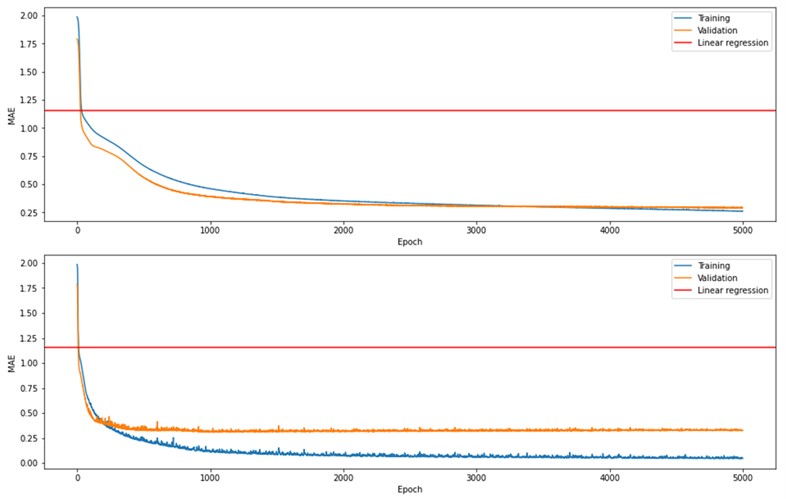
CNN5-7 showed the best results, and they had simple architectures with just one combination of a convolutional, a max pooling and a fully connected layer. CNN13-14 had a more complex architecture with 2 convolutional, 2 max pooling and 3 fully connected layers. Since CNN5-7 and CNN13-14 architectures differ, these top 5 models were chosen to see if a more complex architecture would outperform the simple ones. CNN13 (Fig. 2, bottom) showed overfitting after ~500 epochs, whereas CNN6 (Fig. 2, top) showed a slow but continuous MAE decrease with each epoch.
Fig. 1Validation MAE of all models tested on 8×8 maps
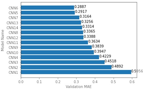
Fig. 2Fitting process of CNN6 (top) and CNN13 (bottom) on 8×8 maps
Considering the top 3 models, CNN7 performed worse with 140096 parameters than CNN6 with 41792 parameters. The model had 3.3 times more parameters, yet MAE was 1.09 times lower. In Fig. 3, CNN6 approximation achieved a 0.23 MAE while linear regression approximation had an 0.89 MAE.
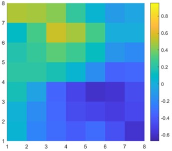
Visually comparing Fig. 3(c) and Fig. 3(d), we clearly see that the CNN approximation is much closer to the TPFA solution, with only the lowest pressure point not being captured correctly, whereas linear regression predicted the corner case better. The difference is better seen in Fig. 4 when we subtract the approximation results from the original solution. The dark red cell of Fig. 4 shows a difference of 1.5 units in CNN6 approximation. However, the linear regression result is overall worse with constant difference of 0.5-1 units.
On the other hand, the top 5 models trained on 16×16 maps showed rather different results. This time, without any changes to the architecture, the more complex models (CNN13-14) outperformed the simpler models (CNN5-7). The difference between the worst complex architecture (CNN14) and the best simple architecture (CNN7) is of 0.2835 MAE (Fig. 5).
Fig. 3Single 8×8 sample solution and approximation results
a) Common logarithm of permeability
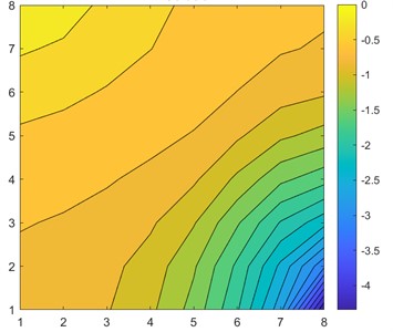
b) TPFA solution
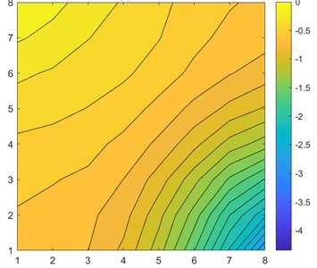
c) CNN approximation
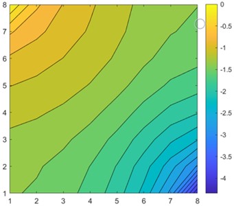
d) Linear regression approximation
Fig. 4a) CNN6 and b) linear regression differences from the original solution
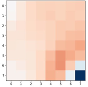
a)
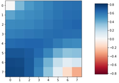
b)
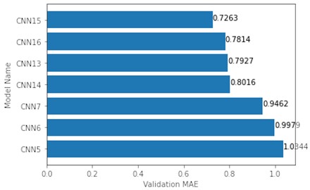
Additional models (CNN15-16) were constructed for map sizes 32×32 and 64×64 to see if architecture complexity could lead to a lower MAE value. Also, despite CNN13 being the best, the number of parameters grows too fast when increasing map size, which leads to a much longer training time. Therefore, new architectures were created, of which the number of trainable parameters would not grow too big. The top 5 and 2 additional models were trained on 32×32 maps and this time the observed trend stayed the same – the more complex architecture, the better approximator it is. The new CNN15 architecture with more hidden layers returned the lowest MAE value of 0.7263, while the lowest MAE value out of the top 5 models was by CNN13 – 0.7927 (Fig. 6). Worth noting is that the new CNN15, which outperforms the CNN13, has 1.6 times less parameters (2823040 and 4565632 respectively).
Fig. 5Top 5 validation MAE of models tested on 16×16 maps
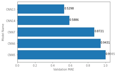
Fig. 6Top 7 validation MAE of models tested on 32×32 maps
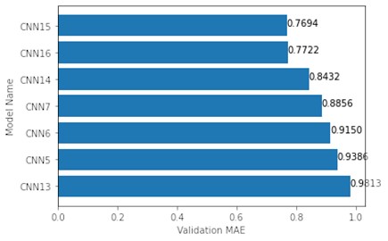
A similar, but with an exception, result was observed with 64×64 data. CNN15 fitted on this dataset once again produced the lowest MAE value of 0.7694. Yet CNN13, which had a top 3 performance with 16×16 and 32×32 maps, returned the highest MAE value of 0.9813 (Fig. 7).
Fig. 7Top 7 validation MAE of models tested on 64×64 maps
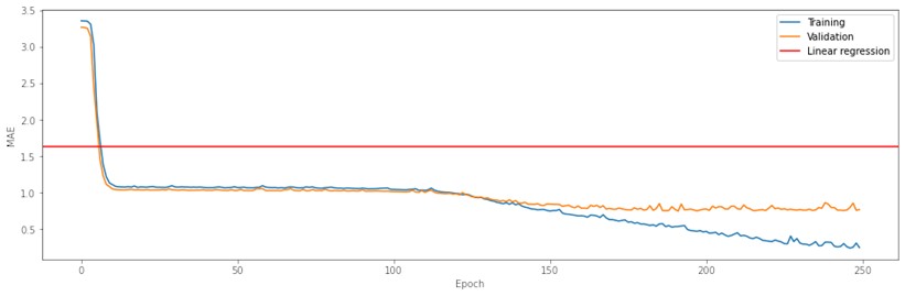
Even though CNN15 returned the best results, the model overfitted – after about 125 epochs validation MAE stopped decreasing, unlike training MAE (Fig. 8). Considering that, a 64×64 map size architecture has over 4.5 million parameters and the output layer needs to predict 4096 values, so it does not come as much of a surprise. Introducing dropout layers between the hidden layers did not increase the performance of our models or helped with overfitting. The experiments with the selected models and their differences in architecture showed, that for this dataset the more complex the architecture, the better prediction will be achieved. However, even the simpler NN models returned considerable results and a higher number of trainable parameters in a model will not guarantee better results.
Fig. 8Training graph of CNN15 (64×64 map size)
5. Conclusions
Simpler CNN architectures produced better results than complex ones on smaller map sizes, but they can only do so much until the variance of data becomes too much to account for.
CNN architectures with several convolutional and fully connected layers gave the best results on higher map sizes. However, the higher variance of the model, the higher chance for the model to overfit.
References
-
A. M. Tartakovsky, C. O. Marrero, P. Perdikaris, G. D. Tartakovsky, and D. Barajas‐Solano, “Physics-informed deep neural networks for learning parameters and constitutive relationships in subsurface flow problems,” Water Resources Research, Vol. 56, No. 5, May 2020, https://doi.org/10.1029/2019wr026731
-
W. Zhang, W. Diab, and M. Al Kobaisi, “Physics informed neural networks for solving highly anisotropic diffusion equations,” in ECMOR 2022, Vol. 2022, No. 1, pp. 1–15, 2022, https://doi.org/10.3997/2214-4609.202244045
-
M. Pal, P. Makauskas, M. Ragulskis, and D. Guerillot, “Neural solution to elliptic PDE with discontinuous coefficients for flow in porous media,” in ECMOR 2022, Vol. 2022, No. 1, pp. 1–17, 2022, https://doi.org/10.3997/2214-4609.202244023
-
L. Shen, D. Li, W. Zha, X. Li, and X. Liu, “Surrogate modeling for porous flow using deep neural networks,” Journal of Petroleum Science and Engineering, Vol. 213, p. 110460, Jun. 2022, https://doi.org/10.1016/j.petrol.2022.110460
-
R. M. Maxwell, L. E. Condon, and P. Melchior, “A physics-informed, machine learning emulator of a 2D surface water model: what temporal networks and simulation-based inference can help us learn about hydrologic processes,” Water, Vol. 13, No. 24, p. 3633, Dec. 2021, https://doi.org/10.3390/w13243633
-
M. Abadi et al., TensorFlow: A System for Large-Scale Machine Learning. tensorflow.org, 2016.
-
D. P. Kingma and J. Ba, “Adam: a method for stochastic optimization,” arXiv:1412.6980, Jan. 2017.
About this article

The authors have not disclosed any funding.
The datasets generated during and/or analyzed during the current study are available from the corresponding author on reasonable request.
Vytautas Kraujalis and Vilius Dzidolikas performed coding and wrote manuscript draft. Mayur Pal provided guidance in formulating problem and methodology for coding the solutions and wrote manuscript draft.
The authors declare that they have no conflict of interest.
