Abstract
Based on Chebyshev’s interpolation theory, the non-homogeneous term of the second-order linear differential equations is interpolated, and a precise integration algorithm with easy programming, high computational efficiency and precision design is realized. The method does not involve inverse operation, and does not need to additionally calculate the matrix index on the integration point, and can control the error boundary based on different precision requirements, so it has high stability and controllability. Numerical examples of periodic loads common in vibration engineering show the effectiveness of the method.
1. Introduction
For the initial value problem of homogeneous linear differential equations with constant coefficients, the matrix index precise calculation method proposed by Academician Zhong Wanxie [1] can increase the calculation of matrix index to computer precision by selecting the integral step size within a reasonable range. This method is widely used in many fields such as random vibration, dynamic response and optimal control. For the processing of non-homogeneous term, Lin Jiahao et al. [2] obtained the analytical solution of Duhamel integral term for the non-homogeneous term of polynomial, periodic function, exponential function and their combination. However, the inverse matrix of the coefficient matrix of the equations is required to be solved. When the coefficient matrix is singular or nearly singular, this method cannot be used, thus greatly limiting its application range and reliability. In order to avoid the inverse operation of the coefficient matrix, Wang Mengfu et al. [3] directly calculates the Duhamel integral by numerical methods. Although such methods can achieve higher precision, the matrix index on the integration point needs to be additionally calculated. Xiang Yu et al. [4] solved the problem by polynomial approximation or Fourier series expansion of inhomogeneous terms. Such methods cannot carry out precision design. If the number of fitting times is higher, the Runge phenomenon will occur. Moreover, as the step size of the integration increases, a large error is generated, so the step size needs to be divided finely, and the amount of calculation is increased.
Based on the Chebyshev’s interpolation theory, this paper interpolates the sampling points of non-homogeneous terms. Different from the traditional uniform sampling, this paper can improve the calculation accuracy based on the Chebyshev interpolation point and avoid the Runge phenomenon. Using the error definition formula, the fitting times can be selected according to different precision requirements, which has strong controllability. Moreover, this method is easy to program and calculate on a computer, and the implementation is simple.
2. Precise calculation of matrix index
Differential equations in vibration engineering, structural dynamic response, etc. can all be transformed into state vector forms:
where is the introduced state vector, is the constant matrix, and is the structural load or control vector. Considering that when 0, the Eq. (1) is transformed into a homogeneous equation, and its solution is:
Let the integration step size , then:
where . It can be known that the relationship between any two adjacent state vectors can be expressed as:
Therefore, the precise calculation of the transfer matrix becomes the core of the solution. In literature [1], the matrix index is processed as follows by using the addition theorem:
Let and the original integration step size become . According to the literature [5], if 20, 0.01, the relative error is 0.151×10⁻¹⁷, which has reached the full accuracy of the computer. This operation ensures the accuracy of the matrix index expansion with Taylor series. Take the first three items of expansion as follows:
where , when calculating with a computer, since the value of is very small, it will become a mantissa when adding with , and thus its original precision is lost. Therefore, it cannot be solved by direct power operation of :
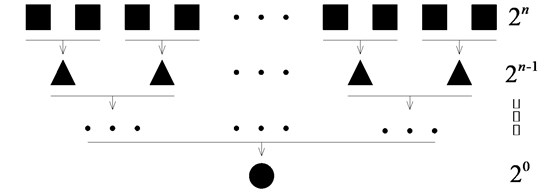
where . So, calculating is equivalent to executing a loop statement:
The principle is shown in Fig. 1. Then execute the following statement at the end of the loop:
Fig. 1Schematic diagram of the loop
3. Chebyshev interpolation approximations
Polynomial approximation is applied to the non-homogeneous term of the differential equations, and the second-order polynomial is taken as an example:
when performing interpolation point sampling, if uniform sampling is performed as described in literature [4], the interpolation polynomial is liable to be twisted near the end of the interpolation interval. As the order increases, the twisting phenomenon becomes more pronounced and the error is greater. It’s the so-called Runge phenomenon.
The Chebyshev interpolation point is a specific optimal point spacing selection method that minimizes interpolation errors. Assuming that Chebyshev interpolation nodes are selected on the interval , , the node coordinates are respectively:
Then use the Newton’s divided difference formula [6] to find the values of the three vectors , , . Extending the approximate polynomial to the original state vector of the differential equation:
Eq. (12) can be solved by the high precision direct integration method of the homogeneous equation described in Eq. (2) to Eq. (9).
4. Precision design
For Chebyshev interpolation, is assumed to be the original function, is a or lower order interpolation polynomial, then points are fitted, and the interpolation error is:
There is an inequality according to Chebyshev’s theory:
where the definition of , , is the same as Eq. (11). Then the maximum interpolation error can be written as:
For example, to perform a polynomial fitting on on [0, 1], it is required to be accurate to 6 decimal places. Through simple experiments, it is found that when 7, the error bound ≈ 0.5715×10⁻⁶, then the sixth-order polynomial fitting can be selected to meet the accuracy requirement.
5. Numerical examples
Differential equations with periodic function as non-homogeneous term:
Analytical solutions when non-homogeneous terms are sine/cosine functions were given in literature [2]:
where and are the coefficient vectors of the sine and cosine functions, respectively. Eq. (17) was verified by Mathematica and the results were consistent. Therefore, the result of Eq. (17) is taken as the exact solution. Introducing the state vector and transforming the Eq. (16) into a first-order differential equation:
Then use the methods in literature [2], literature [1], literature [4] and this paper, respectively, to solve Eq. (18). The integration step 0.01, the fine parameter 20, the results of each method are shown in Table 1 and 2.
Table 1Solution of x1
Step size | Exact solution | Literature [1] | Literature [4] | This article |
0.049179094769134 | 0.048773943800022 | 0.049179261646032 | 0.049179157376206 | |
0.093529329224097 | 0.090431813890316 | 0.093534457158153 | 0.093531255674386 | |
0.128694562148165 | 0.119023415017619 | 0.128730881129231 | 0.128708237262728 | |
0.151217817456480 | 0.130769583117008 | 0.151355950554894 | 0.151269993788613 | |
0.158879713634259 | 0.124766264942132 | 0.159245530921237 | 0.159018459454587 | |
0.150915748723294 | 0.103285473198170 | 0.151666720827195 | 0.151202014701130 | |
0.128091171464306 | 0.071622645861488 | 0.129337190277955 | 0.128569019564925 | |
0.092626109662066 | 0.037498539024419 | 0.094280809634630 | 0.093265231184200 | |
0.047978284706641 | 0.010082245896349 | 0.049539060894824 | 0.048586427269383 |
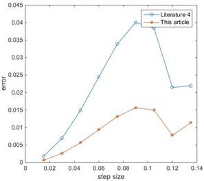
It can be seen from the Fig. 2 and Fig. 3 that because the literature [1] uses a linear approximation, so a large error will occur as the integration step size increases. The error of the literature [4] is close to the error of this paper. This is because the integration step size selected in the above calculation is small, and the larger integration step size is used to compare separately. Take 0.015, repeat the above calculation process, and obtain the error curve comparison between the literature [4] and this paper are shown in Figs. 4, 5.
Table 2Solution of x2
Step size | Exact solution | Literature [1] | Literature [4] | This article |
0.000053759456644 | 0.000053148018043 | 0.000053802149951 | 0.000053775476829 | |
0.000423725534198 | 0.000404520403817 | 0.000425056419986 | 0.000424225882643 | |
0.001395020790211 | 0.001253656462584 | 0.001404688266858 | 0.001398666646464 | |
0.003193642440144 | 0.002623526891556 | 0.003231859612234 | 0.003208116796166 | |
0.005964208798938 | 0.004320682034443 | 0.006071292005589 | 0.006004981148495 | |
0.009755671836064 | 0.005944066131288 | 0.009994373977258 | 0.009847119715415 | |
0.014516394458498 | 0.006944525925839 | 0.014965191794752 | 0.014689486915063 | |
0.020099074451105 | 0.006727765439525 | 0.020832484435684 | 0.020383841886791 | |
0.026275033144355 | 0.004785022016463 | 0.027328318717349 | 0.026686325198872 |
Fig. 2Error of x1
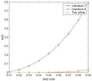
Fig. 3Error of x2
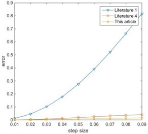
Fig. 4Error of x1 (τ= 0.015)
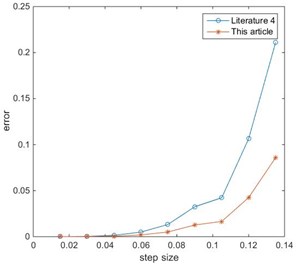
Fig. 5Error of x2 (τ= 0.015)
6. Conclusions
The processing of non-homogeneous terms is the key to solving the differential equations in dynamical systems and vibration engineering. In this paper, the Chebyshev’s interpolation theory is applied to the polynomial approximation of non-homogeneous terms, and an accurate numerical solution can be obtained. The method is stable, and the precision is controllable.
It can be seen from the numerical examples that when the Chebyshev interpolation nodes are used, even if a larger integration step is selected, the error of the method is far less than the error of the literature [4]. And the interpolation order selected in this paper is the same as the literature [4]. If you want to achieve higher precision requirements, you only need to select the appropriate fitting order according to the accuracy design method described in this paper. Therefore, the method can be applied to any non-homogeneous dynamical systems and vibration engineering problems.
References
-
Zhong W. X., Williams F. W. A precise time step integration method. Proceedings of the Institution of Mechanical Engineers, Part C: Journal of Mechanical Engineering Science, Vol. 208, Issue 6, 1994, p. 427-430.
-
Lin J., Shen W., Williams F. W. Accurate high-speed computation of non-stationary random structural response. Engineering Structures, Vol. 19, Issue 7, 1997, p. 586-593.
-
Wang M., Au F. T. K. Assessment and improvement of precise time step integration method. Computers and Structures, Vol. 84, Issue 12, 2006, p. 779-786.
-
Yu X., Yuying H., Jianqiang H. A method of homogenization of high precision direct integration. Journal-Huazhong University of Science and Technology Nature Science Chinese Edition, Vol. 30, Issue 11, 2002, p. 74-76.
-
Xiang Y., Huang Y. Y., Zeng W. G. Error analysis and accuracy design for the precise time-integration method. Chinese Journal of Computational Mechanics, Vol. 19, Issue 3, 2002, p. 276-280.
-
Sauer T. Numerical Analysis. Second Edition, Addison-Wesley, New Jersey, 2012.
About this article

This paper is funded by the International Exchange Program of Harbin Engineering University for Innovation-oriented Talents Cultivation.
