Abstract
A comprehensive study on the application of magneto-rheological (MR) damper in above knee prosthetic is introduced. The stance phase and the swing phase were studied. The knee model was composed of four-bar prosthetic knee mechanism with an MR damper. The equations of motion, of the model, were obtained using Newton's second law at the sagittal plane. To avoid the difficulties of the inverse dynamics, due to the damper’s nonlinear characteristics, a simplified approach was suggested for the Spencer model. This simplified approach was used to calculate the input voltage to the damper to obtain the desirable control force. The input data was obtained from the experimental work by sticking surface land marks to the artificial leg and filming it during performance of the daily activity. The Stream pix, AVI Edit, and WINanalyze software were used to calculate the global kinematics, for the required surface land marks, at each frame of the recorded motion. The model results represent the voltage required for the MR damper, during most daily activities, of a person who uses this kind of an artificial leg. The results showed that the required voltage depends on displacement, velocity and calculated force.
1. Introduction
Walking is human's natural means to move from one place to another. Walking or gait cycle involves the motion of many of the body limbs and joints. Knee plays an important role in the gait cycle. Motion of knee joint is not that simple since it involves planar rolling and sliding motions as well as out of plane motions. Artificial limbs are used to enable amputees to function normally. Above knee artificial leg has not been so successful in the past. A concept and design of polycentric knee arthroplasty based on the biomechanics of normal knee movement was presented by Frank [1]. The diseased articular surfaces of the femoral condyles and tibia plateaus are replaced separately by prosthetic implants secured with cement. A simulation of a total knee joint replacement subjected to a single gait cycle within a knee wear simulator using finite elements was performed by Godest et al. [2]. Bennett and Appoldt [3] measured the loading on an above knee fiber-glass socket by building the socket with incorporated pressure transducers. Unfortunately, their results were accurate only for the single socket used in the experiment. This is because the fact that all modern sockets have different geometries and external loadings due to differences in the amputees. Bielefeldt and Schreck [4] found the difference in loading of four different sockets, during stance, for one patient. Their sockets were, also, built with incorporated transducers. Their results indicated that there is a general trend for the load paths and it can be gauged. Dorious [5] investigated the dynamic response of the human leg in torsion focusing on snow sking injuries. A biomechanical model of the leg system was developed and injury mechanisms to the ankle, knee and tibia were presented. The objective was to determine how torsional leg system dynamics influences injuries of the ankle, knee and tibia under impulse loading. Radcliffe [6] developed a dynamic analysis of above-knee prosthesis during the swing period of the walking cycle. The prosthesis consisted of a four-bar knee mechanism with a pneumatic swing control unit. The kinematics of the knee joint, the dynamics of the leg, and the thermodynamics of the controller were analyzed. Vucina, et al. [7] were concerned with the problem of climbing the stairs by trans-femoral amputee which has not been resolved so far. The difficulty with the problem of upstairs movement of persons with above-knee (AK) prosthesis lies in the need of an external source of energy to enable the user to lift a built in hydraulic cylinder. Their study was dedicated to prove that there is a real possibility for a person with AK prosthesis to climb the stairs. Bae, et al. [8] carried out a dynamic analysis on level walking and stair climbing tasks using musculoskeletal models for normal subjects and above-knee amputees and compared the results with previous studies. According to gait analysis, most of the kinematic parameters showed statistically no difference among the tasks, excluding pelvic tilt, pelvic obliquity, and hip abduction. The activities of major muscles and co-activities of the hamstring and tibialis anterior for the second limb of the amputees showed that the stair ascent task needed more muscle activity than the stair descent task. Nandi and Gupta [9] analyzed the details of the human walk to solve the problem of algorithms lack in instant speed adaptively. They considered stance instability of existing advanced active knee prostheses in a bio- inspired manner and also endeavored various soft-computing techniques being used, presently, in biped locomotion for the use in prosthesis. Akin and Yucenur [10] dealt with the design and testing of an active above knee prosthesis to solve the problem of response to the daily living activities. The essential part of this prosthesis was the knee joint actuator based on active control of basic flexion and extension functions of the knee joint with the motor. The imitation of walking gait pattern by the proposed prosthesis was provided with a trajectory control scheme for the knee joint angle in accordance with the necessity of rule-based control approach. Farahmand, et al. [11] carried out research work to measure and analyze the spatio-temporal variables, the kinematics and, particularly, the net joint moments of the intact and prosthetic limbs of above knee amputee subjects during walking and compared the results with those of normal subjects. The gait characteristics of five trans-femoral amputees and five normal subjects were measured using video-graph and a force platform. Kaufman, et al. [12] employed a crossover design to assess the comparative performance of a passive mechanical knee prosthesis compared to a microprocessor-controlled knee joint in 15 subjects with an above-knee amputation. Objective measurements of gait and balance were obtained. The results showed that subjects demonstrated significantly improved gait characteristics after using the microprocessor-controlled prosthetic knee joint. Hijazi [13] studied the kinematics of the knee joint motion and employed it to determine the most appropriate polycentric knee unit design. Kinematic analysis was performed on three polycentric knee systems. The obtained femur profile and rolling to gliding ratio through flexion for the three systems were compared to the desired femur profile and rolling to gliding ratio. Herr and Wilkenfeld [14] attempted to assess the clinical effects of the user-adaptive knee prosthesis. Kinematics gait data were collected on four unilateral trans-femoral amputees. Using a user-adaptive knee and a conventional, non-adaptive knee, gait kinematic analysis was conducted on both affected and unaffected sides. Results were compared to the kinematics of 12 ages, weight and height matched normal. Zarrugh and Radcliffe [15] investigated the simulation of muscles using MR damper. The Magneto-rheological fluid damper simulates the action of the muscle groups that normally act about the knee joint. Immediately after toe-off, the magneto -rheological fluid damper mimics the quadriceps group; thereby restraining the flexion of the shank and limiting toe rise above the ground. Before heel contact, the magneto-rheological fluid damper provides a hamstring-like action to reduce the angular momentum of the shank, preventing its abrupt impact and subsequent rebound at full extension. Schmalz, et al. [16] used 12 patients with trans-femoral amputations to examine them during alternating stair descent wearing the 3R80, 3C1 and C-Leg knee joints. The results were compared with those of 21 non-amputees. They found that, the electronically controlled hydraulic system of the C-Leg offers more functional advantages than non-electronically controlled hydraulic systems. Porarinsson [17] attempted to investigate the magnetic fields and braking torque in a magneto-rheological (MR) prosthetic knee. The knee used magnetic fields, MR fluid, and thin rotary blades to vary the knee resistance in real time. He pointed out that it is important to investigate the strength of the magnetic fields for different design parameters.
Hua et al. [18] introduced the functional demand of the above-knee prosthesis design. The advantages of the four-bar link mechanism and the magneto-rheological (MR) damper were analyzed in detail. The fixed position of the MR damper is optimized and a virtual proto type of knee joint was given.
The goal of the present study is to determine the input voltage required for the MR damper during most daily activities for the amputee person based on the measured displacements, velocities, accelerations and calculated forces during swing phase period.
2. Analysis
2.1. Model of above knee prosthesis
The artificial knee was modeled as a two- dimensional sagittal plane linkage, consisting of two segments with a four bar mechanism with magneto-rheological fluid damper that simulates the action of the muscle as shown in Figs. 1 and 2. The four bar mechanism has an instantaneous center of rotation (ICR) which has a semicircular pathway located in the femoral condoyle. The instantaneous center of rotation of the socket relative to fixed shank-foot can be located at intersection point (N) of the centerlines of the posterior (EF) and anterior (CD) links.
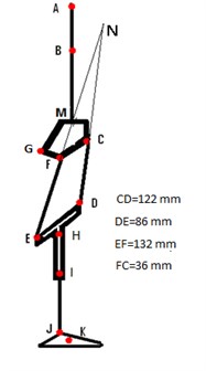
The dimensions of the four- bar knee mechanism were obtained by using instantaneous center of rotation of shank with respect to socket for proper cosmetic appearance and are given in Fig. 2. C, D, E and F are four-bar joints, G and H are damper fixation joints, is mass center of shank segment J is ankle joint K is mass center of foot segment and AM is thigh segment. The angles and thus the angular velocities and accelerations are considered positive in the counter clockwise direction in the plane of the movement, which is essential for consistent use in subsequent kinetic analyses [19].
Table 1 shows the mass of body segments. The controller force () regulates the rotation of the leg to properly prepare it to bear weight at the conclusion of swing phase. The forces in the links (FE) and (CD) pass through the knee center (). In deriving the dynamic equations of the motion it will be convenient to designate points of interest in the mechanism linkage. All vectors passing through the points of interest were referred to an arbitrary fixed coordinate system. The equation of motion of the artificial leg is obtained by applying Newton’s second law at the agitate plane. By taking the moment about the point () for both the external and effective forces:
For the movements like settling on a chair and standing-off from it, the ground reaction force and chair reaction were taken into considerations. The governing equations may then be written as:
Fig. 1The external and effective forces of artificial leg during swing phase
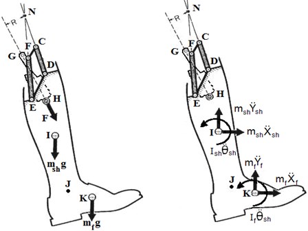
Fig. 2Model of artificial leg and knee four bar mechanism
The damper model of the present study is due to Spencer model [21], see Fig. 3. The equations of this model are:
, are unit vector in -direction and -direction, is damper force vector, and are mass of the shank and the foot respectively, is the Gravitational acceleration, is the vector of normal distance between damper force and point , and are mass moment of inertia of the shank and foot respectively, is the angular acceleration of the shank, and are the total linear acceleration of the mass center of the foot and the shank, , , , are linear acceleration of the shank and foot center in and direction respectively, is the distance vector between points and , is distance vector between points and , and are horizontal and vertical components of the vector , and are horizontal and vertical components of the vector .
The values of the MR damper parameters are listed in Table 2.
Fig. 3Spencer MR damper model used the present
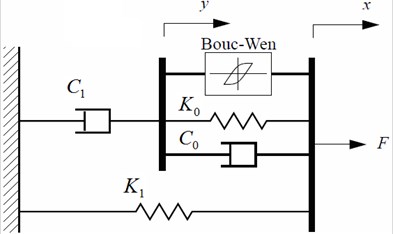
Table 1Body segment mass [20]
Body part | Percent mass |
Head | 6.9 |
Trunk | 46.1 |
Upper arm | 6.6 |
Fore arm | 4.2 |
Hands | 1.7 |
Thights | 21.5 |
Shanks | 9.6 |
Foot | 3.4 |
Table 2Spencer MR damper parameters [22]
Variable | Value | Units | Variable | Value | Units |
784 | N·s/V·m | 2059020 | m-2 | ||
12441 | N/m | 3610 | N/m | ||
1803 | N·s/V·m | 0.024 | m | ||
38430 | N/V·m | 840 | N/m | ||
14649 | N·s/m | 190 | s-1 | ||
136320 | m-2 | 58 | |||
34622 | N·s/m | 2 |
2.2. Inverse dynamic model of MR damper
It has been suggested that the force generated by the MR damper cannot be directly commanded. Only the voltage u supplied to the current driver for the MR damper can be directly changed. A clipped-optimal control algorithm proposed by Dyke et al. [23, 24] is to be used based on acceleration feedback, along with MR damper to approximately generate the desired control force . The command voltage is determined based on how the damper force F is compared to the desired control force and may be written as:
where, is the maximum voltage to the current driver associated with saturation of the magnetic field in the MR damper and is Heaviside step function. However, it was found that the force generated by the MR damper using the clipped algorithm oscillated about the target control force. This was primarily due to the switching of voltage at either its minimum or maximum value.
Tsang and Su [25] proposed an approximate formula based on the Bouc-Wen hysteretic model with the following two assumptions. The external displacement was much larger than the internal displacement . The evolutionary variable was assumed to be equal to its ultimate hysteretic strength (Spencer [26]), i.e.:
Based on the two assumptions, the damper force is:
It can be seen from Eq. (14) that the damper force is a function of the output voltage , the external displacement and the velocity . If the magnitude of the damper force is specified, the output voltage can be obtained at any instant of time:
So the previous equation was putted in a simple quadratic form:
3. Experimental work
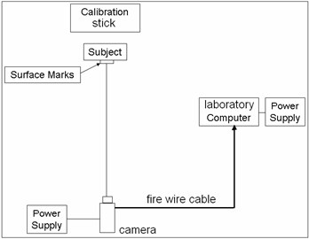
The walking analysis was done by placing twelve visual surface marks on the subject’s body and capturing the 2-D view using a camera placed at a distance behind the subject. The goal of the experiments is to find the position, velocity and acceleration of the surface marks as illustrated in Fig. 2. One healthy male subject (20 years old, 1.8 m and 690 N weight), with no history of knee pain, participated in this experiment. After collecting the positions of the surface land marks three software's were used for extracting their global position at each frame. The First software named, Stream pix, was used to cut the desired motion, from the digital camera, by defining the start and the end of the required motion and to save this motion into a laboratory computer. The second software named AVI edit was used for saving motion pictured from the camera. The third software named WIN analyze was used to track an unlimited number of objects in Video files automatically, and to present the results in almost any desired way (x-y graphs, velocities, accelerations, etc.). The digital video camera used in this study was a JVC, GR-DVX507A. After obtaining the data, the position, velocity and acceleration for the twelve surface marks were fed to a MATLAB program, as well as, the data of the subject. Fig. 4 shows the tracing of three marks F1, F2 and F3 located on the foot of the subject as a sample on the WIN analyze software screen. Fig. 5 illustrates the main components used in collecting the two-dimensional data.
Fig. 4WIN analyze software environment
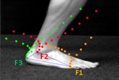
Fig. 5The equipment used in collecting the two-dimensional data
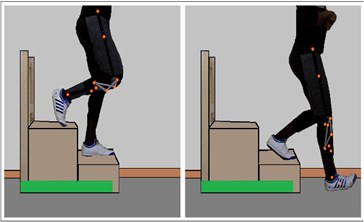
The captured motion was during running. The output from the software as a sample is the displacement of the mark in two dimensional coordinates (, ) with respect to time. The horizontal and vertical coordinates of all marks are shown in Figs. 6 and 7 respectively. Table 3 summarizes the motion during most daily activities of the subject. Some pictures of the experiments are shown from Figs. 8-15.
Table 3The motion of the most daily activities
Motion number | Motion | Motion number | Motion |
1 | Comfortable walking | 7 | Ten-degree ramp descent |
2 | Five-degree ramp ascent | 8 | Fifteen-degree ramp descent |
3 | Ten-degree ramp ascent | 9 | Twenty-degree ramp descent |
4 | Fifteen-degree ramp ascent | 10 | The stairs ascent |
5 | Twenty-degree ramp ascent | 11 | The stairs descent |
6 | Five-degree ramp descent |
Fig. 6Horizontal coordinates of the marks for the foot
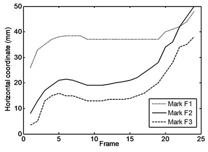
Fig. 7Vertical coordinates of the marks for the foot
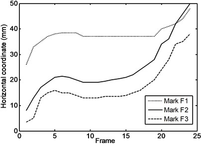
Fig. 8A fully detailed sample of the experiments
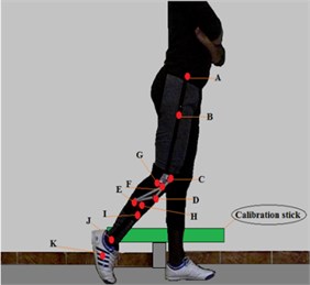
Fig. 9Start and end of comfortable walking motion
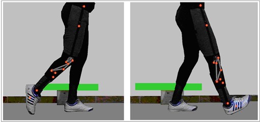
Fig. 10Start and end of ten deg. ramp ascent motion
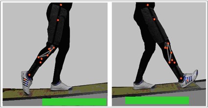
Fig. 11Start and end of twenty deg. ramp ascent motion
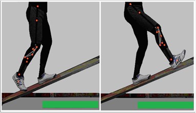
Fig. 12Start and end of fifteen deg. ramp descent motion
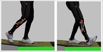
Fig. 13Start and the end of fifteen deg. ramp descent motion
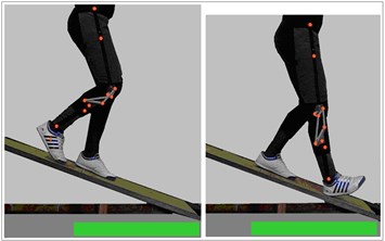
Fig. 14Start and end of stairs ascent motion
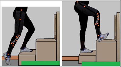
Fig. 15Start and end of stair on a decent motion
3.1. Experimental Set-up
The digital video camera was positioned at a suitable distance according to the required motion of the subject.
Appropriate zoom magnification was set for maximizing the portion of the motion to be captured. The environment had maximum lighting available in order to provide contrast to the surface land-marks color. Shutter speed was set at 30 frames per second to allow enough light for clear definition of the image. The data are to be fed to the inverse model. Iris settings were automatically set to correspond to the shutter speed so as to provide the brightest and clearest image.
Surface marks were secured to the points of interest on the subject as shown in Fig. 2 and then videotaped to identify the subject and to allow the software to recognize the position of the surface land-marks in two dimensions. Once the previous step was performed, the subject performed the motions as shown in Table 3.
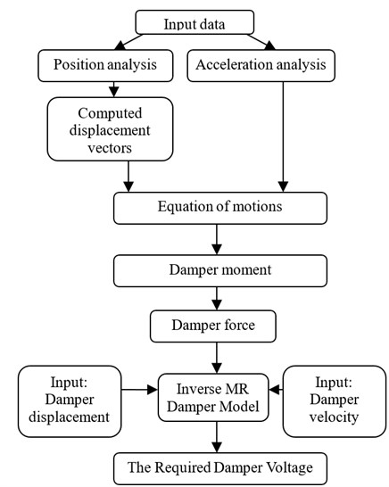
A computer program was designed and developed using MATLAB and SIMULINK software capable of calculating the required voltage during the most daily activities of the person. Fig. 16 shows a block diagram for the software program developed and used in the present study.
Fig. 16Computer program block diagram
3.2. Validations of the Tsang-Su model
The axial damper displacement and axial velocity during comfortable walking (swing phase) is represented by the relative motion between ends of the damper which is represented by marks H and G shown in Figs. 1, 8, and can be obtained from WIN analyze program. Table 4 shows the values of axial damper displacement and axial velocity during comfortable motion.
To examine the assumptions put forward in the Tsang-Su model, two models of MR damper (Spencer and Tsang-Su) were constructed using SIMULINK program. The input displacement to the two models at zero volts is assumed to be harmonic for simplification. The amplitude and frequency of harmonic motion is selected to be 0.008 m and 5 Hz. The selected amplitude and frequency are suitable to give the axial displacement and axial velocity of damper in the range of comfortable walking as listed in Table 4.
Fig. 17 shows the validity of the first assumption which shows that, the value of the external displacement is larger than the value of the internal displacement . Fig. 18 shows the variation of the variable of the two Models which are approximately identical to each other during the cycle. It is to be noted that the value of changed between two fixed values with sharp change at the following times 0.1 s, 0.2 s, 0.3 s and so on till the end of the cycle, and therefore, the value of the force will have a sharp change in its value taking place at the same previous time intervals. Fig. 19 shows the output forces of the two models which are approximately identical to each other during the cycle. This shows that, the MR damper model with the assumptions given above can be used in the present study.
Fig. 17Comparison between the values of x and y in the Spencer model
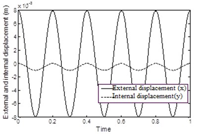
Fig. 18Comparison between evolutionary variable of the two models
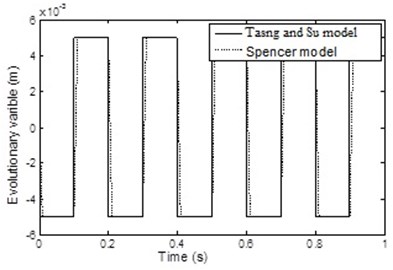
Fig. 19Comparison between the output forces of the two models
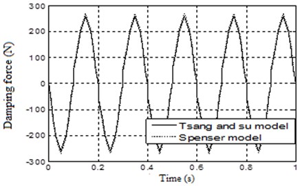
Table 4Axial displacement and velocity of damper during comfortable walking
Swing Time | Axial displacement (m) | Axial velocity (m/s) |
0 | 0 | 0 |
0.1 | –0.0025 | 0.05 |
0.2 | –0.005 | 0.12 |
0.3 | –0.007 | 0.1 |
0.4 | –0.01 | 0.05 |
0.5 | –0.008 | –0.05 |
0.6 | –0.004 | –0.18 |
0.7 | 0.005 | –0.3 |
0.8 | 0.02 | –0.35 |
0.9 | 0.029 | –0.22 |
1 | 0.035 | –0.08 |
4. Input data to the inverse model
The input data required for the inverse dynamic model during most daily activities are not similar. So the full data for the comfortable walking will be clarified first and the rest of the data of the movements are to follow. All data obtained from WIN analyze program are to be fed to the inverse dynamic model which was programmed in SIMULINK software.
4.1. Comfortable walking
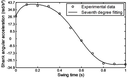
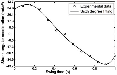
During the swing phase of the patient’s comfortable walking, the shank angle was increased with time from 1.95 to 3.18 rad. at the terminal swing in the manner shown in Fig. 20. The shank angular acceleration is seen to gradually increase from 26.1 to a maximum value of 43 rad/s2 during the period of time of 0.18 seconds from the pre-swing and then begin to gradually decrease and reaches a value of – 32 rad/s2 during 0.9 s at the terminal swing as shown in Fig. 21.
Fig. 20Angular displacement during comfortable motion
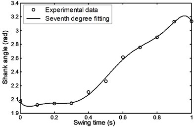
Fig. 21Angular acceleration during comfortable motion
Figs. 22 and 23 show the foot and shank linear acceleration. They start with a slight increase from pre-swing to initial swing and then start to decrease gradually until they reach the mid-swing and then start again to gradually increase until they reach a maximum value at about 90 % of the swing time. The so called evolutionary variable depends on the parameters whose adjustment allows shaping the linearity of the control during unloading and the smoothness of the transition from the pre-yield to post-yield area as well as the axial damper velocity as shown in Fig. 24. It is an indication to the axial damper velocity sign change.
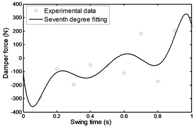
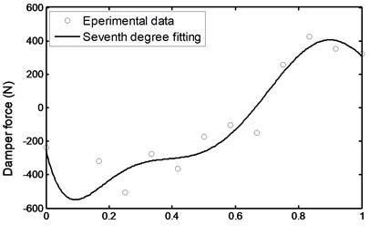
The damper force as observed from the equation of motion, (see Eq. (1)) depends on inertia torque, inertia forces of shank and foot and their distance from the instantaneous center of rotation and other parameters like the weight of the shank – foot system and their distance from the instantaneous center of rotation. But from the comparison of all previous parameters it is obvious that the value and the nature of the force depend mainly on the values of the inertia forces as shown in Fig. 25.
Fig. 22Linear acceleration of the foot during comfortable motion
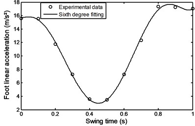
Fig. 23Linear acceleration of the shank during comfortable motion
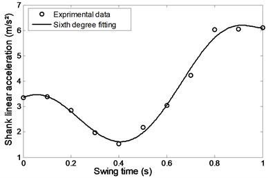
Fig. 24Evolutionary variable during comfortable motion
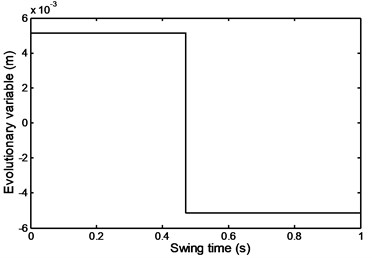
Fig. 25Average damper force during comfortable motion
4.2. Ramp ascent and descent
Figs. 26-31 represents the input data during ramp assent at different inclinations. Figs. 26 and 27 show the individual angular position and angular acceleration for the shank during the various ramp inclinations. Figs. 28 and 29 show the linear acceleration for the foot and shank during the various ramp inclinations respectively. Figs. 30 and 31 show individual and average axial damper force for various ramp inclinations. In a similar fashion, Figs. 32 to 35 represent the input data during ramp descent at different inclinations.
Fig. 26Angular position for the shank during ramp ascent
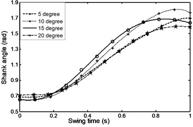
Fig. 27Angular acceleration for the shank during ramp ascent
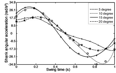
Fig. 28Linear acceleration for the foot during ramp ascent
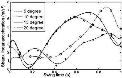
Fig. 29Linear acceleration for shank during ramp ascent
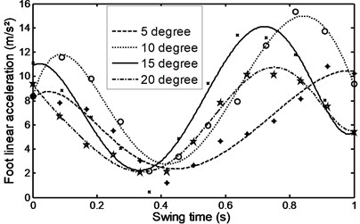
Fig. 30Average damper force during ramp ascent
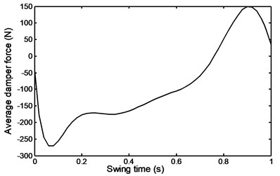
Fig. 31Angular position for the shank during ramp descent
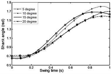
Fig. 32Angular acceleration for the shank during ramp descent
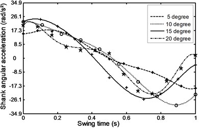
Fig. 33Linear acceleration for the foot during ramp descent
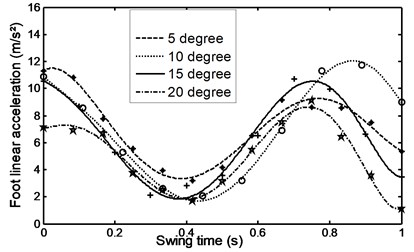
Fig. 34Linear acceleration for the shank during ramp descent
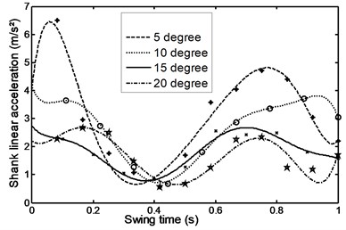
Fig. 35Average damper force during ramp descent
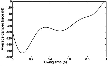
Fig. 36Angle of the shank during stairs ascent
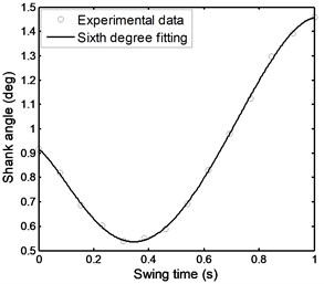
Fig. 37Angular acceleration of the shank during stairs ascent
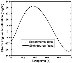
Fig. 38Linear acceleration of the foot during stairs ascent
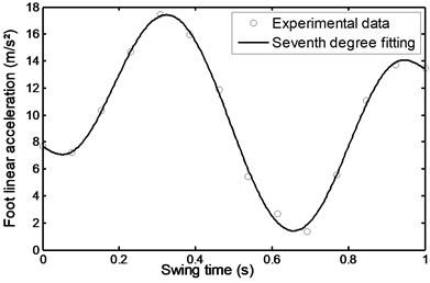
Fig. 39Linear acceleration of the shank during stairs ascent
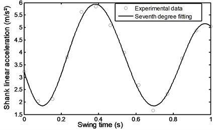
Fig. 40Evolutionary variable during stairs ascent
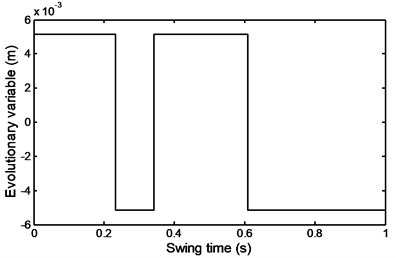
Fig. 41Damper force during stairs ascent
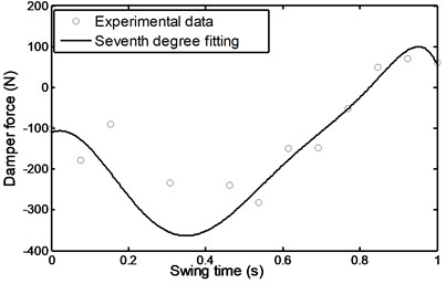
Fig. 42Angle of the shank during stairs descent
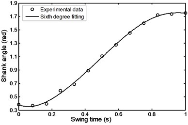
Fig. 43Angular acceleration of the shank during stairs descent
4.3. Stairs ascent and descent
Figs. 36 to 41 represent the input data during stairs ascent.
Figs. 42 to 47 represent the input data during stairs descent.
Fig. 44Linear acceleration of the foot during stairs descent
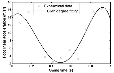
Fig. 45Linear acceleration of the shank during stairs descent
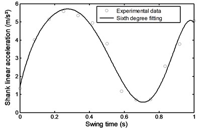
Fig. 46Evolutionary variable during stairs descent
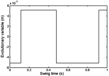
Fig. 47Damper force during stairs descent
5. Results and discussions
The results and their discussions are to be made for the different walking conditions starting with the case of comfortable walking. The results are to deal with the voltage obtained from the simulation and are to be fed to the MR damper in order to give the prescribed motion and appropriate damping force during the wing time inspects. It is clear that this voltage depends on the required displacement, acceleration and the damping force.
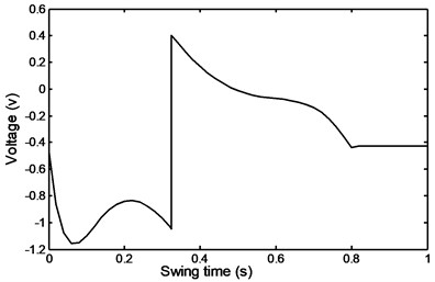
Starting by the comfortable walking zone, Fig. 48 shows the required damper voltage which decreases and then increases gradually in the beginning of the cycle following the trend of the damper input force.
It is noted that irrespective of the local sudden change in the voltage appearing at approximately 0.47 s of swing time the voltage continues to increase gradually and decreases again till the end of the swing time. This shows that the effect of ubrupt change in the voltage has no considerable effect on the damping force. This may be attributed to the low rate of momentum transfer due to the smallness of the masses involved.
The damper voltage required during a ramp ascent is shown in Fig. 49. It can be seen that from the beginning of the swing time till a value of 0.325 s, where the same ubsrupt change in damper velocity takes place that, the voltage follows the trend of the required damper force behavior. From the ubrupt sudden increase in voltage till the end of the period the voltage decreases gradually until it reaches an asymptotic value of – 0.425 V.
Fig. 48Comfortable walking voltage
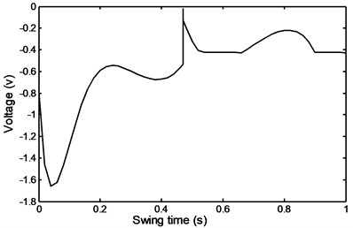
Fig. 49Ramp ascent voltage
The abrupt rise in voltage may be attributed to the larger average rate of momentum required during a ramp descent and is in general in qualitative agreement with that of ramp ascent as can be seen from Fig. 50.
It is seen that disregarding the small zone ahead of swing time 0.035 s the voltage follows the same trend as the required average damping input force.
The required damper voltage is also shown in Figs. 51 and 52 for cases of stairs ascent and descent respectively.
Fig. 50Ramp descent voltage
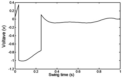
Fig. 51Stairs ascent voltage
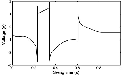
Fig. 52Stairs descent voltage
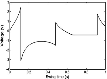
The qualitative agreement on the behavior of the voltage for both cases is clear and in general follows the trend of the required damper forces as can be seen from Figs. 43 and 47.
From the foregoing discussion it can be seen from the results of the required voltage that it follows in general the same trend as that of the input damper force irrespective of the type of motion.
6. Conclusions
This study introduced a dynamic model of artificial knee for the amputee person. The knee is formulated from a four bar mechanism connected by a Magneto –rheological damper to control the motion of the amputee person during most daily activities. Also the present work studies the input voltage required for the MR damper based on the displacement, velocity, acceleration and force during swing phase period. The value of input voltage is important for the damping force and moment to achieve the realistic and comfortable motion or any activity for the amputee person. Such a model can be used for improving the mechanical design of the artificial knee, both by suggesting improvements of the MR damper itself and by understanding the relation between an applied voltage and the time dependent damping force of the knee during motion.
From the experimental work and analysis of the presented results the following conclusions are drawn,
1) The voltage required for MR damper to cope with most daily activities is always following the trend of the damping force.
2) The variation of the voltage over the swing time for comfortable motion case is relatively small and has a maximum of order 1.6 V which is tractable by simple control units.
3) For the case of ramp ascent and decent the maximum change in voltage is of order 1.5 V for both cases and close to the comfortable motion case.
4) The variation of the voltage for stairs ascent and descent over the swing time does not exceed the order of 2.5 V for both cases and as far as the case of control in concerned it matches with the other cases of motion considered.
References
-
Gunston Frank H. Prosthetic simulation of normal knee movement. The Bone and Joint Journal, Vol. 53, 1971, p. 272-277.
-
Godest A. C., Beaugonin M., Haug E., Taylor M., Gregson P. J. Simulation of a knee joint replacement during a gait cycle using explicit finite element analysis. Journal of Biomechanics, Vol. 35, Issue 2, 2002, p. 267-275.
-
Appoldt F. A., Bennett L. A preliminary report on dynamic socket pressures. Bulletin of Prosthetics Research, Vol. 67, 1967, p. 20-55.
-
Bielefeldt A., Schreck H. J. The altered alignment influence on above knee prosthesis socket pressure distribution. International Series on Biomechanics, Vol. 2, 1981, p. 387-393.
-
Dorious L. K. Errors in alignment of center of pressure and foot coordinates affect predicted lower extremity torques. Journal of Biomechanics, Vol. 17, Issue 1, 1984, p. 1-9.
-
Radcliffe C. W. Biomechanics of knee stability control with four-bar prosthetic knees. ISPO Australia Annual Meeting, Melbourne, 2003.
-
Vucina A., Hudec M., Raspudic V. Kinematics and forces in the above-knee prosthesis during the stair climbing. International Journal of Simulation Modeling, Vol. 4, Issue 1, 2005, p. 17-26.
-
Bae T. S., Choi K., Hong D., Mun M. Dynamic analysis of above-knee amputee gait. Clinical Biomechanics, Vol. 22, Issue 5, 2007, p. 557-566.
-
Nandi G. C., Gupta B. Bio-inspired control methodology of walking for intelligent prosthetic knee. Scientific Commons, 2008.
-
Akin O. K., Yucenur M. S. Design and control of an active artificial knee joint. Mechanism and Machine Theory Journal, Vol. 41, Issue 12, 2006, p. 1477-1485.
-
Farahmand F., Rezaeian T., Narimani R., Dinan H. P. Kinematic and dynamic analysis of the gait cycle of above knee amputees. Scientia Iranica, Vol. 13, Issue 3, 2006, p. 261-271.
-
Kaufman K. R., Levine J. A., Brey R. H., Iverson B. K., Crady S. K., Padgett D. J., Joyner M. J. Gait and balance of transfemoral amputees using passive mechanical and microprocessor-controlled prosthetic knees. Gait and Posture, Vol. 26, Issue 4, 2007, p. 489-493.
-
Hijazi A. L. Knee Joint Kinematics and its Applications in Prosthetics Limbs Design. M.S. Thesis, Wichita State University, 1998.
-
Herr H., Wilkenfeld A. J. User-adaptive control of a magneto-rheological prosthetic knee. Industrial Robot: An International Journal, Vol. 30, Issue 1, 2003, p. 42-55.
-
Zarrugh M. Y., Radcliffe C. W. Simulation of swing phase dynamics in above-knee prostheses. Journal of Biomechanics, Vol. 9, Issue 5, 1976, p. 283-292.
-
Schmalz T., Blumentritt S., Jarasch R. A comparison of different prosthetic knee joints during step over step stair descent. The American Academy of Orthotists and Prosthetists, Vol. 3, Issue 3, 2007.
-
Porarinsson E. P. Analysis of Magneto-Rheological Prosthetic Knee. M.S. Thesis, University of Iceland, 2006.
-
Xie Hua-Long, Liang Ze-Zhong, Li Fei, Guo Li-Xin The knee joint design and control of above-knee intelligent bionic leg based on magneto-rheological damper. International Journal of Automation and Computing, Vol. 7, Issue 3, 2010, p. 277-282.
-
Winter D. A. Biomechanical and Motor Control of Human Movement. Second Edition, Wiley and Sons, New York, 1990.
-
Churles A., Ronuld W. Human Survival in Aircraft Emergencies. NASA C.R., National Aeronautics and Space Administration, Washington D.C., 1969.
-
Spencer J. B., Dyke S. J., Sain M. K., Carlson J. D. Phenomenological model of a magneto-rheological damper. Journal of Engineering Mechanics, Vol. 123, Issue 3, 1997, p. 230-238.
-
Liao W. H., Lai C. Y. Harmonic analysis of a magneto-rheological damper for vibration control. Smart Materials and Structures, Vol. 11, Issue 2, 2002, p. 288-296.
-
Dyke S. J., Spencer Jr. B. F., Sain M. K., Carlson J. D. Seismic response reduction using magneto rheological dampers. Proceedings of the IFAC World Congress, San Francisco, CA, 1996.
-
Dyke S. J., Spencer Jr. B. F., Quast P., Sain M. K., Kaspari Jr. D. C., Soong T. T. Acceleration feedback control of MDOF structures. Journal of Engineering Mechanics, Vol. 122, Issue 9, 1996, p. 907-918.
-
Tsang H. H., Su R. K. L., Chandler A. M. Simplified inverse dynamics models for MR fluid dampers. Engineering Structures, Vol. 28, Issue 3, 2006, p. 327-341.
-
Spencer B. F. Reliability of Randomly Excited Hysteretic Structures. Springer-Verlag, New York, 1986.
Cited by
About this article

Attia E. M. suggested the model and planned for the experimental work, performed the dynamic equation of the model, analyzed the data from experimental work, constructed and arranged the manuscript to be ready for publication. Abd El-Naeem M. A, performed the dynamic equation of MR damper model and its inverse, take the pictures during the experimental work by camera, constructed the computer programs, collected the references. El-Gamal H. A, revised the text especially the results and discussion, performed the conclusions. Awad T. H., revised the text and computer programs, commented on computer program block diagram. Mohamed K. T., revised the dynamic equation of the model, revised the text and references, commented on the design of experimental work.
