Abstract
Loss factor is one of the most significant parameters of Statistical Energy Analysis (SEA) which represents the damping loss characteristics of a system and indicates the ability of its vibration energy consumption. In order to estimate it, the power input method (PIM) and the impulse response decay method (IRDM) have become widely used especially when the object of study is made of Fiber Reinforced Plastics (FRP) of which dynamic interaction is really complicated. Numerical simulation is also applied to analyze the loss factor of the spring-damping-system with single degree of freedom (SDOF) using MATLAB to introduce the identification procedure of PIM and IRDM. With the comparison of the methods, the analytical study indicates these techniques are effective for the estimation of loss factor. This paper focuses on an experimental approach to get the SEA loss factor of FRP plate and the test investigations are performed in detail. The requirements and limitations of each method applied are discussed and PIM is a better solution dealing with this kind of the composite material. The loss factor of test specimen is obtained to provide a valuable reference for the prediction and control of vibration and noise of yachts with SEA.
1. Introduction
Modern yachts are usually manufactured with the material of fiber reinforced plastics (FRP) which possesses the advantage of light, stiff, conductive and corrosion resisting. It is important to accurately predict the levels of vibration and noise at the design phase considering the high manufacturing cost of yachts. Statistical Energy Analysis (SEA) has become a powerful way of solving the problem above since it was originally and systematically mentioned by Lyon in 1975 [1]. This method could predict the averaged response levels of a subsystem in view of energy with relative accuracy. But during applying the SEA on a system, loss factor is required to describe the ability of energy dissipation of a subsystem. It is considered as a significant parameter getting an accurate model of SEA which has a great influence on the results of prediction. The complex structure of FRP plate leads to the fact that investigating the loss factor analytically is very difficult. Experimental measurement is normally taken as a more effective way of obtaining this parameter. Generally, the methods of loss factor estimation could be classified as two kinds:
1) Power based loss factor estimation techniques which includes Power Input Method (PIM) and Half-Power Bandwidth Method (HPBM).
2) Decay rated loss factor estimation techniques which include Reverberation Decay Method (RDM), Random Decrement Technique (RDT) and Impulse Response Decay Method (IRDM).
Between the power based methods, PIM is one of the most widely methods used as an experimental way of determining loss factor. And the result of this method is independent of natural frequencies which is suitable for the wide frequency band averaged loss factor estimation [2]. A series of researches of PIM are taken by M. Carfagni. His studies consist of three parts: numerical investigation [3]; experimental investigation with impact hammer excitation [4]; experimental investigation with shaker excitation [5, 6]. In order to measure the damping characteristics of a vehicle side glass quickly and accurately, a practical application of PIM is presented by B. Bloss [7]. K. De Launghe discusses the process of obtain SEA parameters and the influence of the chosen excitation and response points during PIM measurement [8]. Some significant problems of applying PIM are also discussed by A. Dande [9]. The loss factor determines the time of damping out when a system is applied on an impulsive or an interrupted stationary excitation. RDM, RDT and IRDM are the representative techniques on the basis of decay rate methods. The core idea of IRDM is replacing the output response by the impulse response of system. In the papers of Mark S. Ewing and his team, the methods above are taken to estimate the loss factors [10-14]. Panels with and without damping treatments are usually discussed to evaluate the methods in experimental and computational analyses.
In this work, two widely-used techniques of different kinds (PIM and IRDM) are taken to estimate the loss factor for FPR plate of yachts. Numerical simulation of spring-mass system with PIM and IRDM is carried out to be in comparison and the analytical study indicates the availability of estimating the loss factors by these methods. Experimental setups and procedures are introduced in detail and the differences and limitations of each method used for estimation are discussed which could be beneficial to the study of the prediction and analysis of complex structures made of the composite materials.
2. Fundamental theory
2.1. Power input method
The loss factor of a system per cycle in the frequency band centered at could be defined as:
where, is the loss factor, is the frequency band center, is the energy dissipated from damping and is the strain energy.
Under a steady state condition, the input energy is equal to the dissipated energy when the input energy stays at a establish location, so can be replaced with :
where, is the input energy.
However, these two kinds of energy: and could not be measured by experiment method directly. So the force and velocity at the point where the energy inputs to the system needs post-processing [15-18]. Therefore is taken as:
where, is the driving point mobility function and is the power spectral density (PSD) of input force.
And when calculating , three assumptions should be considered [7].
1) The strain energy is replaced as twice as the kinetic energy:
where, is the kinetic energy.
2) The volume integral is estimated with a limited number of velocity measurements distributed over the whole system to evaluate the kinetic energy. The system is approximated by a summation when system is divided into equal portions which makes the kinetic energy could be calculated by:
where, is the number of measurement points, is the mass of the portions and is the PSD of the velocity response of each measured point .
3) The system is assumed as a linear one which allows that:
where, is the transfer mobility function.
Taking all the three assumptions above into account, the measurement locations should be uniformly spread over the system where the mass and of each portion is equal. Eq. (1) could be approximated by combing Eq. (3), (5), (6) as:
All the necessary terms to obtain loss factor in Eq. (7) could be experimentally determined directly. It is considered that PIM could be performed by measuring the input force and velocity response at the driving locations. So the accuracy of FRF of each point is the decisive factor of loss factor estimation. This method introduces the steps of measuring loss factor of a SEA model which could be used for the purpose of prediction of noise and vibration.
To satisfy the requirements of SEA model, the loss factor with several driving points should be evaluated with Eq. (7). And the band average loss factor is computed as:
where, is the number of driving points.
2.2. Impulse response decay method
IRDM is one of the decay rate methods which are on the basis of the measurement of the initial decay rate with the excitation form of an impulse or an interrupted stationary excitation [19]. The response amplitude of the system or structure at time domain would decay at a slope proportional to shown in Fig. 1. The decay rate is equal to when the energy of system is proportional to the peak amplitude squared. So the decay rate of two points at time domain in decibels is [20]:
where, and is the time of point 1 and 2, is the frequency, is the loss factor, and is the peak amplitude of the response of system at and .
DR is defined as the decay rate below:
where, is the amplitude variation of exponential decay curve in the time of which is:
where, is the cyclic frequency in radians/seconds as . So:
and loss factor which is equal to could be in decibels:
From the Eq. (13), the loss factor is proportional to the decay rate DR while to the frequency of system inversely. Solving loss factor for a single modal resonance or averaged one of many modal resonances for frequency band, the decay rate is the most significant parameter.
Fig. 1Transient response of a single degree of freedom system
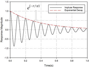
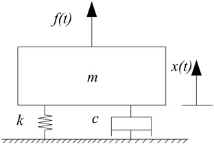
Fig. 2Single degree of freedom system
3. Numerical analysis
Analytical model of simple spring-mass-damper system which is the simplest among the vibratory systems is created with assumed values of different loss factors. Then PIM and IRDM are separately applied on the system to obtain the simulated values. The numerical simulation shows both methods provide effective loss factor values which match the assumed ones in acceptable error range. The system consists of three elements: spring (elastic element), mass (inertia element), and damper (damping element) as illustrated in Fig. 2.
The general form of the differential equation of the system under forced vibrations is:
where, is the mass of system, is the position of mass, is the viscous damping rate of system, is the stiffness of system, is the external dynamic load of system, is the initial displacement and is the initial velocity.
As for the is the unit impulse, the response replaced by of which is usually called unit impulse response. The solution of Eq. (14) under this condition is [21]:
where, is the unit impulse response, is the natural frequency and is the damping ratio.
When an impulse occurs at , the solution of Eq. (15) becomes:
As for the case of zero initial conditions, the solution of Eq. (14) is given by:
Eq. (17) states that the response of any linear system with any exciting force is the convolution integral of the unit impulse response and the input force.
3.1. Power input method
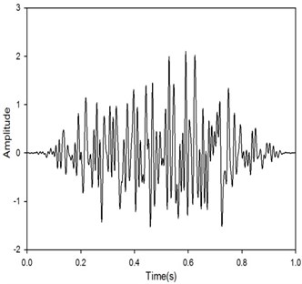
To estimate loss factor with a shaker, the random force is usually taken as the excitation of the system. The software of MATLAB is used to generate random signals as driving force of the single degree of freedom system which is represented in Fig. 3. In order to reduce the leakage of random signals, a Hamming window is applied on the force in Fig. 4. And the parameters of system are assumed in Table 1. The loss factor of system is 0.0158 given by .
In the case of SDOF, PIM indicates that the structural loss factor could be calculated of the way which compares dissipated energy (replaced by total input energy) to the structure's strain energy (replaced by kinetic energy). The input energy of system is given by and the kinetic energy given by . So the expression of loss factor of SDOF system is [13]:
where, is the input force of SDOF and is the velocity response of SDOF.
Table 1Simulated parameters of single degree of freedom system by PIM and IRDM
Parameter | Method | |
PIM | IRDM | |
1 Kg | 0.75 Kg | |
0.5 Ns/m | 0.75 Ns/m | |
1000 N/m | 500 N/m | |
31.6228 | 25.8199 | |
0.0079 | 0.0194 | |
Time resolution | 0.001 s | 0.001 s |
Time period | 1 s | 1 s |
Fig. 3Random driving force
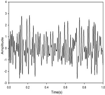
Fig. 4Filtered random force
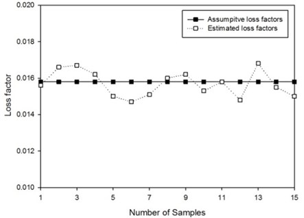
Thus the expected loss factor is 0.0158 of the simulation. 15 samples of loss factor calculation of SDOF system by MATLAB codes are taken to compare with the supposed value illustrated in Fig. 5. The result indicates the estimated loss factors by PIM is accurate at the level of which the variation between the estimated values and 0.0158 is 6.3 % at most.
Fig. 5Estimation of loss factors by PIM of SDOF
3.2. Impulse response decay method
The measurement of the initial slope of the decay of linear system subject to initial excitations needs to be tested to apply IRDM [22]. For this system subjected to zero initial displacement and velocity, the loss factor could be estimated by two main steps:
1) Get the Hilbert transformation of the impulse response.
In order to obtain the exponential decay, the Hilbert transformation is used in Fig. 6. The loss factor could be determined from the decay rate of the exponentially decaying envelope of impulse response approximately obtained by the magnitude of Hilbert transformation [14]:
where, is the unit impulse response stated in Eq. (15) and is the Hilbert transformation of .
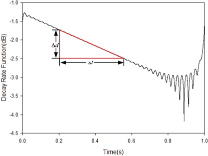
2) Get the logarithmic decrement of the Hilbert transformation.
The impulse response signal needs to be plotted as log-rms amplitude at time domain which is easy to determine the decay rate. From Fig. 7, the system of single mode and a constant loss factor, the decay rate is:
where, is the decay time and is the change of magnitude of decay curve in the time of .
Fig. 6The impulse response and its envelop of SDOF
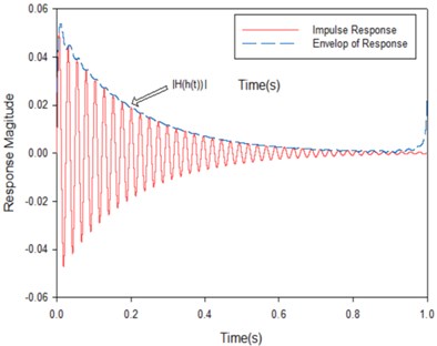
Fig. 7The decay rate function of SDOF in dB
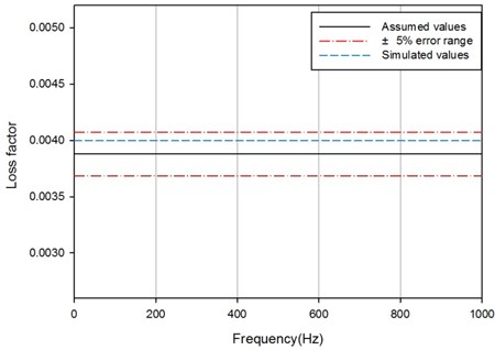
All the parameters of SDOF are simulated in Table 1, so the constant loss factor is 0.0388. The response of SDOF is defined as the convolution integral of the unit impulse response and the input force shown in Eq. (17). Then the Hilbert transformation is applied on the impulse response to get the exponentially decaying envelope. Finally, the logarithmic decrement of the Hilbert function is calculated to get the loss factor shown in Fig. 8. More times of simulation are carried out and the simulated values match the assumed ones well with no more than 5 % error which could be concluded that comparing to PIM, IRDM is more steady and accurate to estimate the loss factor of a single and well-defined modal resonance system like SDOF although the early decay rate is lack of accuracy and should be ignored.
Fig. 8Estimation of loss factor by IRDM of SDOF
4. Experimental setup and procedures
The experiments with PIM and IRDM are taken to estimate the loss factor of SEA parameters which could be beneficial to the further study of prediction of vibration and noise levels of modern yachts. For the investigation, the FRP plate weighted 2.73 kg, manufactured by Xiamen Hansheng Yacht building company and 500×500×28 mm in size is chosen in the study. In order to keep the stable damping property while the tests are taken, the atmospheric conditions especially the parameter of temperature are controlled by two air conditioners. The specimen is suspended by two nylon ropes to create free-free boundary condition as explained in Fig. 9. The ropes are arranged symmetrically to ensure the plate is in the horizontal plane with a gradienter. The other end of ropes is tied to a firm frame of aluminium.
Fig. 9Experimental setup of PIM
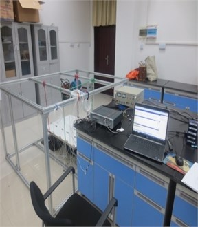
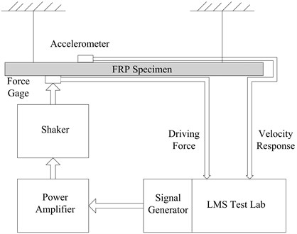
Fig. 10Schematic of experimental setup of PIM
With the number of portions increasing, the curves of loss factor will stabilize asymptotically [5]. But due to the limit of experiment conditions, only a limit of number of sections are taken in the estimation experiments. The cover of plate is divided into 16 portions, and 16 measuring points which should be distributed equally of the whole structure are located at the center of each portion in Fig. 11. The vibration responses of specimen such as the velocity response and the FRFs are measured at these points. In order to investigate the influence of the locations of excitation to the quality of estimated loss factor of PIM, eight driving points are random selected with MATLAB codes and the sensors placements shown in Fig. 12.
Fig. 11Locations of driving points and measuring points
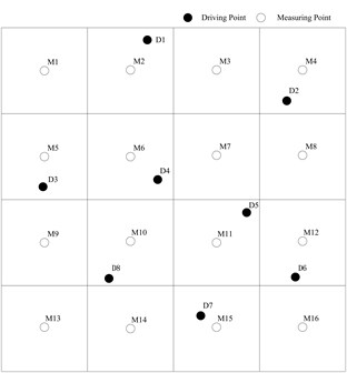
Fig. 12Sensors placements
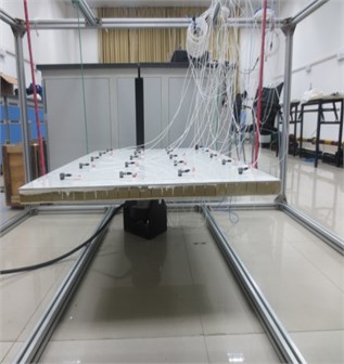
The significant influence of “added mass effect” should be minimize by using the light PCB single-axial accelerometers, model 333b30, weighted about 0.14 oz. It is no doubt that the mass distribution of structure is affected by the sensors, the negative quality is defined on each measuring point of model created by the modification prediction module of LMS Test lab. HEV-200 shaker of high-energy and electro-dynamic is used to generate the driving force. And HEA-200C power amplifier is used to match it. A PCB 208C02 force sensor is connected to the shaker with a flexible and thin stinger. And the gage is connected to the base side of the specimen at the driving points to measure input forces to obtain of the input energy.
The data transfer mobility spectrum could not be measured directly. So the velocity response of the other side is picked by an accelerometer on the opposite of the driving point. Because of the upper limit frequency of shaker, the plate is excited from 0 Hz to 4 KHz via a signal generator of LMS Test lab. All the input and response signals are measured by an LMS SCADA-III front end. And LMS Test lab 14A is used to collect and analyze the date. And then they are transferred for the loss factor calculation with MATLAB.
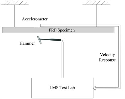
While applying IRDM, the kinds of excitation method are usually relatively free because steady driving with a shaker or transient with a hammer is feasible. In this work, hammer excitation with model 086C02 of PCB is chosen and the choice of hammer tip should be cautious. As the hard one could excite a wider range of frequencies than the soft, another matter is trying to avoid double hits when driving at an excitation point with the hammer which could be reminded by the noise created by test software. The plate is divided as the PIM experiment and the response FRFs are measured. Figs. 13 and 14 present the schematic and experimental setup of this method.
Fig. 13Experimental setup of IRDM
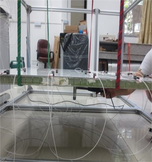
Fig. 14Schematic of experimental setup of IRDM
5. Test results
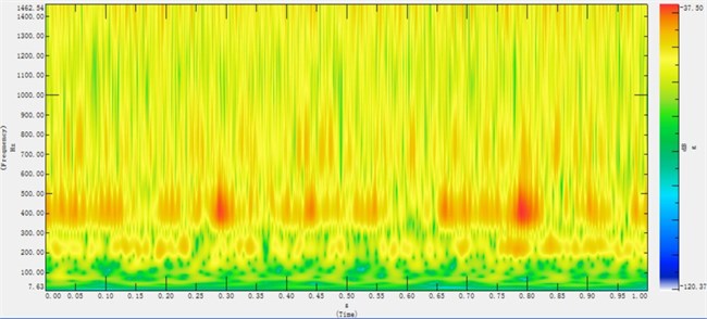
To estimate the loss factor of the FRP specimen accurately, all the original data needed are obtained and analyzed in the LMS test lab 14A. The FRFs of eight different driving points are measured and the acceleration response at the 16 measurement points are acquired by experiments. The acceleration response of M7 with the driving point 4 verse time is shown in Fig. 15. The wavelet transformation is used to indicate the time-frequency relationship of this signal in Fig. 16, the lack of modal resonances leads to the low amplitude from 0 to 150 Hz around. And the high amplitude zone between 200 to 500 Hz indicates the low capacity of energy dissipation which could result in the high loss factor in the frequency band. Then the integral calculation and power spectrum density (P.S.D) operation are taken in the post-processing tool of test lab to get the P.S.D. of velocity response at the measurement locations for PIM and the P.S.D. of input forces at the chosen input locations are also tested. According to the Eq. (8), the loss factors of different situations are calculated.
Fig. 17 shows the loss factor under the condition of 1 Hz frequency resolution, white noise random force excitation, at driving point 4. The loss factor of the FRP is much higher than the steel which is used as the traditional material of ship building whose values are about 1-6×10⁻⁴ [23-27] from the test results. The trend is same as other loss factor of materials by PIM which decreases in damping with increasing frequency. The lower loss factor values around 500 Hz are influenced obviously by the FRF of excitation point illustrated in Fig. 18.
Fig. 15The acceleration response of driving point 4
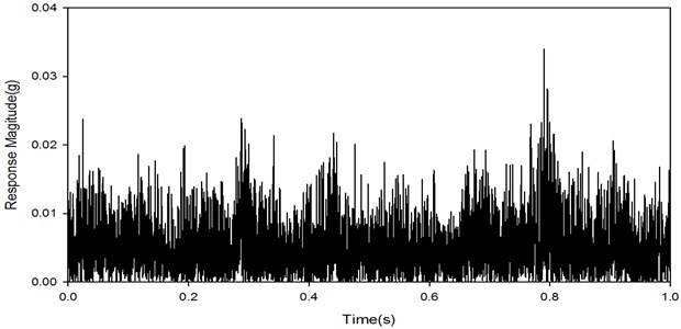
Fig. 16The wavelet transformation of M7 with the driving point 4
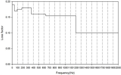
As the result of practical limitation on experimental conditions, only a limited number of driving points are chosen to determine the loss factor values. The results of estimation of driving point 1,5 are shown in Fig. 19. It is obviously proved that the excitation locations influence the estimation of loss factor greatly. The driving point 1 is located around the edge, and the tendency of this curve is of great oscillation and away from the normal values which could not be an effective result. Some more driving points at edge and corner are also carried out, but several results even fail. So a conclusion could be drawn that while applying PIM, the locations of excitation should avoid at edges and corners, the points near the center and arbitrary locations are recommended. And after the elimination of the unsuccessful driving points like D1, the averaged loss factor values are represented in Fig. 20 of which indicates that the loss factor of FRP plate in the experiments is around 0.15.
For a complex structure of many modes of vibration driven by an impulse excitation, the impulse response is difficult to identify. The inverse Fourier Transform (IFFT) of the FRFs are usually taken to get the decay rate. And the function should be plotted a log-rms scale with the time of linear scale. Besides the two steps mentioned in section 3.2, Figs. 21-23 suggest the procedure of the estimation of loss factor using IRDM for the FRP plate which is based on these main steps: Firstly, get the FRFs of interested frequency bands. For each FRF of tested points, the segment FRF of the frequency band of interest like the center frequency 500 Hz with the band from 400 to 630 Hz; Secondly, IFFT is applied on each segment FRF to obtain the impulse response; Finally, plot the response signal on a logarithmic amplitude scale with time in linear scale to obtain the initial decay rate in decibels. All the steps should be repeated for the frequency bands of measured FRFs. And the loss factor of IRDM is plotted in the Fig. 24 on the averaged decay slope of all the FRFs.
Fig. 17Estimation of loss factor at driving point 4
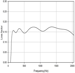
Fig. 18The FRF of driving point 4
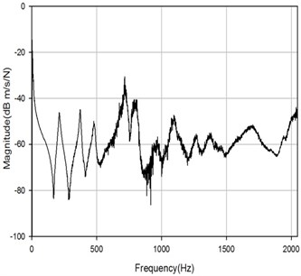
Fig. 19Comparison of loss factor of driving point 1, 5
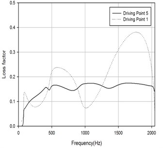
Fig. 20Averaged loss factor of reliable driving points
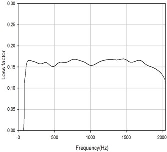
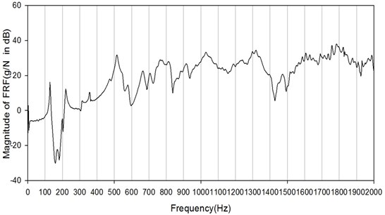
Fig. 21The FRF of tested sheet of M10 by D8 from 0-2000 Hz in decibels
From the schematic of experimental setup of different methods in Figs. 10 and 14, IRDM is a simply technique with only response signal tested while PIM need to record the input and response data. The main limitation of IRDM is that this method is only suitable for a single and well-defined modal resonances or averaged frequency bands across many modal resonances. Fig. 24 indicates that the loss factor of IRDM appear to be overestimated in the low frequency band with no or only a few modes. Comparing to this, PIM does a better job when no modal resonances in a frequency band. With the high loss factor plate of FRP, there are a number of oscillation of the decay curve of IRDM before it becomes easy to get the decay rate. Manual slope fitting must be taken and the human courses could lead to errors. So the initial decay rates of response are quite difficult to attain accurately. If the response points are a little far from the excitation point, the FRF of these points could not be obtain clearly with the reason of high loss factors. On the basis of these reasons, PIM is a recommend to an appropriate method of estimation for the FRP plate.
Fig. 22The FRF of tested sheet of M10 by D8 in the 1/3 octave band centered on 500 and 1000 Hz in decibels
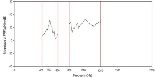
Fig. 23Schematic diagram of the decay curve after IFFT of FRFs for the frequency center of 63 Hz

Fig. 24Averaged estimation of loss factor of IRDM
6. Conclusions
To determine the loss factor for a FRF plate of yacht, experimental techniques of the power input method and the impulse response decay method are investigated. With an analytical model of SDOF, both ways of estimation are compared with the simulated values. Both methods are proved to be reliable and convenient ways of the determining loss factors. For the composite materials with high loss factors like FRP plate, PIM is a better choice of estimation technique than IRDM with great influence of human errors. In addition, it is extremely useful of confirming of dynamic responses and noise levels of numerical models for complex structures. And the loss factor obtained by experiments with the constant values of 0.15 of the whole frequency band could be used for the further study of prediction and analysis of vibration and noise levels of luxury yachts.
References
-
Lyon R. H. Statistical Energy Analysis of Dynamical Systems: Theory and Applications. M.I.T. Press, Cambridge, USA, 1975.
-
Bloss B., Rao M. D. Estimation of frequency-averaged loss factors by the power injection and the impulse response decay methods. The Journal of Acoustical Society of America, Vol. 117, Issue 1, 2005, p. 240-249.
-
Carfagni M., Pierini M. Determining the loss factor by the power input method (PIM). Part 1: numerical investigation. Journal of Vibration and Acoustics, Vol. 121, Issue 3, 1999, p. 417-421.
-
Carfagni M., Pierini M. Determining the loss factor by the power input method (PIM). Part 2: numerical investigation. Journal of Vibration and Acoustics, Vol. 121, Issue 3, 1999, p. 422-428.
-
Carfagni M., Citti P., Pierini M. Determining the loss factor using the power input method with shaker excitation. Proceeding of the 16th IMAC, CA, 1998, p. 585-590.
-
Wei W., Fan X., Song H., et al. Imperfect information dynamic Stackelberg game based resource allocation using hidden Markov for cloud computing. IEEE Transactions on Services Computing. 2016.
-
Bloss B., Rao M. D. Measurement of damping in structures by the power input method. Experimental Techniques, Vol. 26, Issue 3, 2002, p. 30-32.
-
LaungheK. De, SasP. Statistical analysis of the power injection method. The Journal of. Acoustical Society of America, Vol. 100, Issue 1, 1996, p. 294-303.
-
Dande H. A., Ewing M. S. On the effect of mechanical excitation position on panel loss factor estimation with the power input method. Proceeding of the Internoise ASME NCAD Meeting, 2012, p. 1-12.
-
Wei W., Xu Q., Wang L., et al. GI/Geom/1 queue based on communication model for mesh networks. International Journal of Communication Systems, Vol. 27, Issue 11, 2014, p. 3013-3029.
-
Mark S. Ewing, Himanshu Dande, Kranthi Vatti Validation of panel damping loss factor estimation algorithms using a computational model. 50th AIAA/ASME/ASCE/AHS/ASC Structures, Structural Dynamics and Material Conference, 2009, p. 1-30.
-
Himanshu Amol Dande Panel Damping Loss Factor Estimation Using the Random Decrement Technique. University of Kansas, Kansas, 2010.
-
Kranthi Kumar Vatti Damping Estimation of Plates for Statistical Energy Analysis. University of Kansas, Kansas, 2011.
-
Himanshu Amol Dande Evaluation of Loss Factor Estimation Techniques for Free Hanging Flat Panels Excited Mechanically. University of Kansas, Kansas, 2013.
-
Plunt J. The power injection method for vibration damping determination of body panels with applied damping treatments and trim. SAE Transactions, Vol. 100, Issue 6, 1991, p. 1563-1571.
-
Li J. Q., He S. Q., Ming Z. An intelligent wireless sensor networks system with multiple servers’ communication. International Journal of Distributed Sensor Networks, Vol. 7, 2015, p. 1-9.
-
Zhu Z., Xiao J., Li J. Q., et al. Global path planning of wheeled robots using multi-objective memetic algorithms. Integrated Computer-Aided Engineering, Vol. 22, Issue 4, 2015, p. 387-404.
-
Lin Q. Z., Chen J. Y. A novel micro-population immune multiobjective optimization algorithm. Computers and Operations Research, Vol. 40, Issue 6, 2013, p. 1590-1601.
-
Bloss B., Rao M. D. Estimation of frequency-averaged loss factors by the power injection and the impulse response decay methods. The Journal of Acoustical Society of America, Vol. 117, Issue 1, 2005, p. 240-249.
-
Lyon R. H., DeJong R. G. Theory and application of Statistical Energy Analysis, 2nd ed. Butterworth-Heineman, Newton, MA, 1995.
-
Norton M. P. Fundamentals of Noise and Vibration Analysis for Engineers. Aviation Industry Press, Beijing, China, 1993.
-
Bloss B., Rao M. D. A Comparison Between Power Injection and Impulse Response Decay Methods for Estimating Frequency Averaged Loss Factors for SEA. SAE Technical Paper, 2003-01-1566.
-
Yao D. Y., Wang Q. Z. Fundamentals and Applications of Statistical Energy Analysis. Beijing Institute of Technology Press, Beijing, China, 1995.
-
Wong K. W., Lin Q. Z., Chen J. Y. Error detection in arithmetic coding with artificial markers. Computers and Mathematics with Applications, Vol. 62, Issue 1, 2011, p. 359-366.
-
Lin Q. Z., Zhu Q. L., Huang P. Z., Chen J. Y., Ming Z., Yu J. P. A novel hybrid multi-objective immune algorithm with adaptive differential evolution. Computers and Operations Research, Vol. 65, 2015, p. 95-111.
-
Du Z. H., Zhu Y. Y., Liu W. X. Combining quantum-behaved PSO and K2 algorithm for enhance gene network construction. Current Bioinformatics, Vol. 8, Issue 1, 2013, p. 133-137.
-
Wei W., Yang X. L., Shen P. Y., et al. Holes detection in anisotropic sensornets: topological methods. International Journal of Distributed Sensor Networks, Vol. 21, Issue 9, 2012, p. 3216-3229.
Cited by
About this article

This work is supported by the Fundamental Research Funds or the Central Universities (3132014338) and Educational Commission of Liaoning Province of China (L2015066) financially.
Yannian Cai designed the experiments, performed the data analyses and wrote the manuscript. Hongliang Yu contributed to the conception of the study and helped perform the analysis with constructive discussions. Bingnan Liang contributed to analysis and manuscript preparation and performed the analysis of the power input method. Yuchao Song helped design the experiments and performed the analysis of the impulse response decay method. Jin Yan contributed to the experimental equipment and helped perform the experiments.
