Abstract
Steel catenary riser (SCR) is one of the most popular and economic risers in the development of deep-water oil and gas field. As a difficulty in the SCR design, the pipe-soil interaction at the touchdown zone is affected by the soil strength, riser diameter, upper floating body, and other factors. Conventionally, the pipe-soil interaction was mainly studied based on the static response of the riser under a linear seabed which was inconsistent with the actual situation. Therefore, a dynamic characteristic model was built in the paper for more realistic simulation of the pipe-soil interaction. And experiments were conducted to verify the reliability of the numerical model. Based on the verified model, the dynamic process of the nonlinear time-domain was analyzed. Different parameters, such as the soil strength and dynamic loads, were changed to analyze their effects on the pipe-soil interaction in the whole process which provided a certain foundation for the SCR design.
1. Introduction
In recent years, the oil and gas exploration has gradually turned to the deep-water area with the exhaustion of the oil and gas resources in shallow water. And the traditional rigid riser is no longer applicable because the operating depth increases [1]. As one of the relatively economy risers in the deep-water oil and gas development [2], SCR is often connected to SPAR, FPSO, semi shallow platform and other floating platforms rather than jacket and other fixed platforms which are inapplicable to the deep-water exploration, which could be explained by the greater dynamic load by SCR due to the motion of the upper floating body [3]. The touchdown point (TDP) as the connection point of the riser and seabed, is the most fatigue zone [4]. An ideal seabed model needs to be built in order to estimate the TDP fatigue of the riser more accurately. According to the groove distance and pipe-soil interaction process proposed by Bridge [6], Aubeny [5] firstly proposed an un-attenuated P-y curve of the seabed soil body. Although the loading state of the riser at all stages can be described, the P-y curve cannot explain the impact of the repeated uplifting of the riser on the soil stiffness [7]. By considering the attenuation of the seabed stiffness, You [8] obtained a P-y curve that can better simulate the complex loading condition. The initial model of the simplified seabed was proposed by Jung [9] to simulate a seabed-pipe which was as a flexible tube supported by a series of linear spring. Similarly, Dunlap [10] also simplified the pipe-soil interaction to the riser and placed it on a series of springs; the soil stiffness was simulated by a linear P-y curve. The elasticity of the soil spring was obtained by the finite element method, and the deflection and bending stress of the riser was obtained by the finite element and differential methods. The seabed models were mostly linear elastic in the mentioned researches. Though the pipe-soil interaction can be directly reflected, the linear elastic seabed model cannot describe the groove, nonlinear soil stiffness, soil suction, pipe-soil separation, seabed soil deformation, seabed soil attenuation and other complex problems [11-13]. A dynamic characteristic model was built in the paper for more realistic simulation of the pipe-soil interaction. And experiments were conducted to verify the reliability of the numerical model. Based on the verified model, the dynamic process of the nonlinear time- domain was analyzed. Different parameters, such as the soil strength and dynamic loads, were changed to analyze their effects on the pipe-soil interaction in the whole process, which provided a certain foundation for the SCR design.
2. 2Dynamic characteristic description of pipe-soil interaction
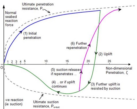
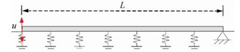
The common form of the model was shown in Fig. 1. The model started from the initial penetration, as shown in blue lines of the figure. With the increase of the penetration depth, the resistance asymptotic line was close to the extreme penetration reaction force .
However, the soil body effect was decreased rapidly at the maximum initial tangent rigidity when the riser penetration stopped and the reaction force uplifted. And the soil reaction force was turned to the suction force with the continuous uplifting of the riser. The maximum suction force was approaching the extreme suction force . The extreme penetration reaction force was controlled by the . And the soil suction force was decreased to 0 with the further increase of the riser. After the completion of a complete uplifting process of the penetration, the soil body resistance curve penetrated the riser again, thus reflecting the attenuation condition of the soil stiffness. The re-penetration depth of the soil body was larger than the original penetration depth which was controlled by the parameter . Then, the pipe-soil zone was penetrated and separated by the riser along the envelope curve.
Fig. 1Soil model characteristics in different stages
3. The pipe-soil interaction model and basic theories
3.1. Basic theories
The schematic diagram of steel catenary riser and micro-segment was shown in Fig. 2. The seabed was horizontal, the water depth was and the riser was anchored at point . Only the form of the riser on a two-dimensional plane was considered, and three-dimensional deformation was neglected. Only the horizontal component and constant velocity were considered. The tension of the riser was at point , the angle between the force direction and -axis was . The tension of the ship at the anchor point was , and the angle between the force direction and horizontal direction was . The weight of riser unit length in water was , and the length of pendency segment of the riser was . The anchor point of the riser on the seabed was taken as the coordinate origin to build a rectangular coordinate system. The catenary micro-segment with a length of was extracted.
Fig. 2Schematic diagram of riser and micro-segment
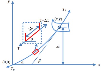
Tensions at both ends of the micro-segment were and . The angle between the force direction and -axis was . Its self-weight in water was . Tension was the continuous function of , whose projection at -axis and -axis were also continuous functions. After expanding the two projection functions respectively into Taylor series and ignoring the second-order, the projection of tension at the -axis was obtained as follows [14-16]:
The projection of tension at -axis was as follows:
Eq. (1) was the tension in the horizontal direction, and Eq. (2) was the tension in the vertical direction. In the other end, the tension can be also decomposed into two tensions in the horizontal and vertical direction, respectively. The horizontal tension was , and the vertical tension was . In addition, the micro-segment will bear a gravity in the vertical direction. Moreover, the micro-segment was balanced in the horizontal and vertical direction. As a result, the balanced equation of the micro-segment can be written as follows:
The following differential equations could be obtained from Eqs. (3) and (4):
The following boundary conditions could be obtained from Fig. 2:
According to Eqs. (7) and (8), the differential Eq. (5) can be solved. As a result, the riser equation under the general condition could be obtained as follows:
In case of 0, the equation could be simplified as follows:
According to the above mathematical formula, the coordinate and tension of pendency segment of the riser at any point could be obtained when the water depth, top angle and horizontal tension were known.
3.2. Pipe-soil interaction model
In the analysis, the selected riser was a steel riser pipe, which had a total length of 800 m, outer diameter of 0.35 m, inner diameter of 0.25m, elastic model 2.05×10¹¹ kPa, material density of 7850 kg/m3. The depth of the riser in the water was 500 m, the top of the riser was connected to the upper platform through a hinged method and its end was anchored on the seabed. The anchor point of the riser was set as the coordinate origin, the coordinate of anchor point was (500, 0, 0) and the coordinate of the hung point was (0, 900, 0). The heave motions of only the upper floating body were considered in the analysis, with the amplitude of 1 m, 2 m and 3 m, respectively, and the period of 10 s. The seabed was horizontal. The soil with the low, medium and high intensities was selected, and their shear strengths were 2.8 kPa, 3.1 kPa and 3.4 kPa, respectively. The corresponding shear strength gradients were 1.6 kPa/m, 1.8 kPa/m and 2.0 kPa/m, respectively. Finally, the pipe-soil interaction model was built, as shown in Fig. 3.
The model of the riser was divided into 2 segments. The former 500 m of the riser was the pendency segment which was out of touch with the soil. The segment was relatively sparse, and the length of each segment was 3 m. The later 300 m of the riser was the touchdown segment. The segment was relatively fine, and the length of each segment was 1 m. The finer the touchdown segment was, the higher the computational accuracy was, which had higher requirements for computers. The previous research results were combined with those of this paper to make a comparison. When the segment was 1 m, the computer could be fully used, and the analyzed error was smaller.
Fig. 3Pipe-soil interaction model
Fig. 4Schematic diagram of OrcaFlex linear element
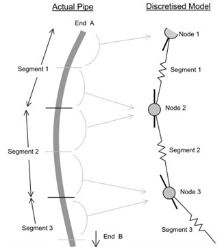
The SCR was welded by many steel pipes with a certain length. The dimension in the length direction was larger than the dimension of its cross section, and it belonged to a very long structure. Therefore, this paper used beam element to simulate the riser. OrcaFlex software was used in the numerical analysis, and the riser was analyzed by the line element in the software. Featured with the spring system of axial stiffness and bending stiffness, it could be applied to simulate the cables, chains and other structures. The line element was a series of mass points which were connected through the mass-less spring. The mass points were considered as nodes, the springs between node connections were called as a segment, and each segment was a line element as shown in Fig. 4. The real pipeline was shown in the left side while the OrcaFlex model was shown in the right side.
In the touchdown segment in Fig. 4, nonlinear spring elements which were connected with the ground were set on the nodes of the riser as shown in Fig. 5. In order to research it, the wave direction was assumed to be the same as the flow direction, and the incident angle was 180°. The wave was propagated along the -axis, spring elements in the vertical direction were only set on the touchdown segment.
Fig. 5Pipe-soil interaction model in touchdown segment
In the finite element analysis, the penalty function and Lagrangian multiplier method were used to solve the dynamic contact effect between the riser and seabed, and analyze the influence regulation of dynamic contact effect on normal contact pressure stress, tangential contact shear stress and tangential slip.
The contact between the riser and seabed was a surface-to-surface contact. The touchdown zone was ( was the riser pipe diameter). Compared with the pipe diameter, the touchdown zone of model analysis was large enough. The influence of the seabed boundary conditions was neglected. In the numerical simulation, actual risers were steel. The sectional dimension of the riser was smaller than its length. In addition, the linear model in the paper was the riser. The stiffness of the riser was greater than that of soil. In the contact process, the deformation of the riser was dimensionless compared with the displacement of soil. Therefore, the riser was defined as a linear rigid body. In this case, the interaction between the riser and the seabed could consider the displacement and contact force of the riser rather than the riser deformation, which saved the computational time and improved computational efficiency. In the analyzed process, the soil was considered as a nonlinear model because the seabed soil would have great deformation under the acting force of the riser due to its small stiffness. Through the interaction between the riser and the seabed soil, the nonlinear result of soil could be transferred to the linear riser.
The corresponding bending moment would happen to the riser which was under the acting force of the seabed soil. Due to the bending moment, the section of the riser would change from a circle into an ellipse. However, the change of the riser section was not considered in case of conducting a simulation because the ratio between the length and section of the riser was in ocean engineering. The researched object of this paper was the interaction between the riser and seabed soil. The riser was defined as a rigid body. Therefore, the change in the section of the riser could be neglected compared with the length of the riser, which had no influence on the researched object of this paper. Thus, this paper ignored the change of the section in the analyzed process.
Nine kinds of conditions were applied in the paper to study the impact of different seabed strengths, motions of the floating body and other factors on the pipe-soil interaction in the touchdown zone as shown in Table 1.
Table 1Detailed description of nine kinds of conditions
Conditions | Shear strengths | Shear strength gradient | Heave amplitude | Heave cycle |
1 | 2.8 kPa | 1.6 kPa/m | 1 m | 10 s |
2 | 2.8 kPa | 1.6 kPa/m | 2 m | 10 s |
3 | 2.8 kPa | 1.6 kPa/m | 3 m | 10 s |
4 | 3.1 kPa | 1.8 kPa/m | 1 m | 10 s |
5 | 3.1 kPa | 1.8 kPa/m | 2 m | 10 s |
6 | 3.1 kPa | 1.8 kPa/m | 3 m | 10 s |
7 | 3.4 kPa | 2.0 kPa/m | 1 m | 10 s |
8 | 3.4 kPa | 2.0 kPa/m | 2 m | 10 s |
9 | 3.4 kPa | 2.0 kPa/m | 3 m | 10 s |
4. Verification for dynamic characteristics of pipe-soil interaction
As the pipe-soil interaction process was relatively complex, the subsequently results cannot be ensured without the experimental verification for the accuracy of the numerical model.
Fig. 6Distribution of test equipment in NGI model
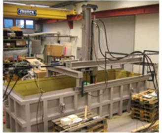
a) NGI test model
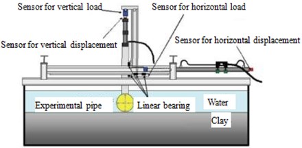
b) Distribution of NGI test equipment
Fig. 7Comparison of experiment and simulation for soil resistance curve
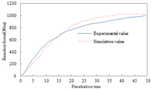
NGI equipment was applied in the experimental, and the size of the experimental chamber was 17 m×3.6 m, as shown in Fig. 6. A two-axis hydraulic loading system was adopted in the experimental process to realize the vertical load of the riser. The outer diameter of the tested riser was remained consistent with that of the simulated one, namely 0.35 m. In addition, the roughness processing was carried out on the outer surface of the model. The seabed clay was used as the experimental soil, and the static load and vacuum drainage were applied in the experimental box to re-consolidate the soil which was placed for one month. Since the test was conducted indoors, the depth of water was limited and only resistance curves with penetration depth of less than 50 mm could be tested. Then the experimental results were compared with the numerical simulation results as Fig. 7. It could be seen that the experiment and simulation were close in terms of both the trend and numerical value, indicating that the established pipe-soil model herein was reliable and could be used for a subsequent analysis.
5. Analysis of dynamic response for SCR
5.1. Dynamic characteristic comparisons of pipe-soil interactions
The traditional analyses were mostly based on the linear seabed model which was inconsistent with the actual situation. Two different situations of linear and nonlinear seabed models were analyzed in the paper. Motions with the heave amplitude of 2 m were selected, and the analytical length was 2400 s.
Fig. 8Touchdown zone shape of riser at deepest penetration zone
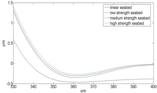
Fig. 8 was the form of SCR under gravity, buoyancy and tension, and it was also the initial form for the further analysis of the riser. The initial form of SCR generally used the catenary method for solving the problem. The catenary method was described through the catenary equation with considering bending stiffness to obtain the initial equilibrium form of SCR. The seabed with low, medium and high strengths in Fig. 8 was a nonlinear seabed. As shown in the figure, the penetration depth of SCR increased with the length before 350 m for 4 kinds of seabed. When the length was 350 m to 360 m, the penetration depth change of SCR was not obvious. However, the penetration depth gradually decreased for 4 kinds of seabed when the length was more than 360 m. When the length was 360 m for 4 kinds of seabed, the penetration depth of SCR was the maximum. In case of adopting the linear seabed, the penetration depth of the riser into the seabed was obviously greater than that under a nonlinear seabed. When the penetration depth of the riser into the seabed increased, the overall falling degree increased. 3 kinds of nonlinear seabed were compared. With the increased strength of the seabed soil, the penetration depth of SCR decreased but they basically kept the same change trend. In addition, the penetration depth of the seabed with low intensity was close to that of the linear seabed.
The above computational model was taken as a basis and 0.1 s was considered as a computational time step. If the computational time step was too large, the singular point in the figure could be neglected. However, a small time step would increase the load of computers. Finally, the computed coordinate (the seabed was taken as the base level) of the deepest penetration point under each time step during 1000 s to 1500 s was extracted to draw a time-history curve of the dynamic displacement of the linear seabed and low strength seabed as shown in Fig. 9. From Fig. 9, it could be seen that the time-history curve of SCR under the linear seabed presented obvious periodicity and the penetration depth of SCR was about –0.3 m. Under a low strength seabed, the amplitude of displacement slightly changed and demonstrated the periodicity. The penetration depth of SCR was about –0.2 m. The response amplitude of displacement under a low strength seabed was smaller than that under a linear seabed. In addition, 2 kinds of seabed kept the same response cycle of the displacement. At the same time point, the penetration depth of SCR under a linear seabed was obviously greater than that under a low strength seabed.
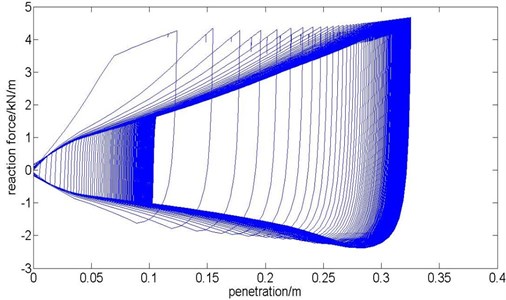
Only the soil resistance curve under the penetration depth less than 50 mm was studied in Fig. 9. And the soil resistance curve of the whole process was obtained under the circumstance of the low-intensity soil in Fig. 10. It could be seen that at the touchdown zone, the P-y curve penetrated to the deepest point was also changed cyclically under the effect of the cyclic load. After the stabilization of the motions, the P-y curve path was also repeated.
Fig. 9Time-history curve of dynamic displacement
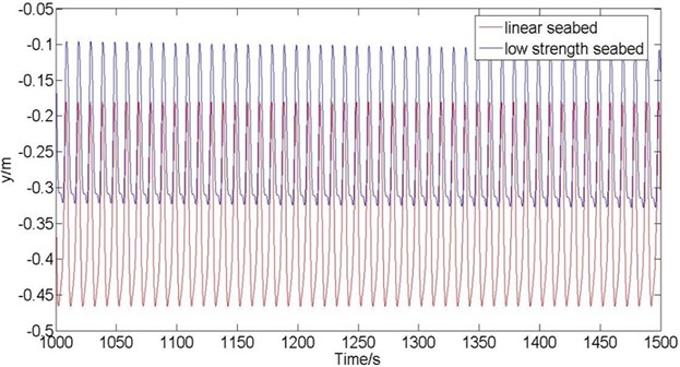
Fig. 10P-y curve
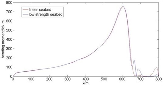
Under two different seabed conditions, the time-history figure of the dynamic bending moment at the deepest penetration point in the interval of 1000 s-1500 s was shown in Fig. 11. It could be indicated that the trends and changing of two curves were basically the same under different seabed types, while the maximum value of the nonlinear seabed bending moment was greater than that of the linear seabed. The heave cycle of 10 s was chosen throughout the analyzed process. Therefore, a maximal value of the bending moment would be appeared on the riser at any point in the 10 s. In the interval of 1000 s-1010 s, the changes of the riser along the length direction were selected under the maximum bending moment, whose result was shown as Fig. 12. It could be seen that the trends of the riser bending moment along the length direction were basically the same under different seabed strengths, namely, both increasing first, decreasing then and reaching their maximal value at the touchdown area. It was found from the comparison of Fig. 11 and Fig. 12 that the maximum riser bending moment was in the touchdown area of riser and seabed rather than the deepest penetration point. Seabed was in conformity with such a law.
Fig. 11Time-history curve of dynamic bending moment
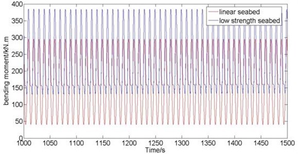
Fig. 12Distribution diagram of riser bending moment along length direction
5.2. Effect of floating body on dynamic characteristics of pipe-soil interaction
The medium-strength seabed soil was applied for the analysis in this section. The heave amplitude of the upper floating body was 1 m, 2 m and 3 m, respectively and the heave cycle was 10 s, namely 4, 5 and 6 conditions in Table 1. The penetration depth of the riser, touchdown zone shape and bending moment were analyzed under various external incentives, and the effects of external load on the dynamic performance of the riser were compared.
Fig. 13Touchdown zone shape of riser
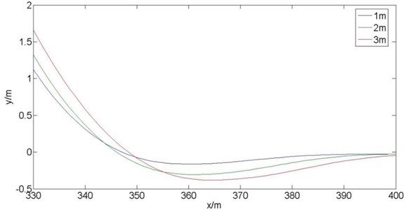
The touchdown zone shape of the riser under various external incentives was shown in Fig. 13. It was indicated that the greater the heave amplitude of the upper floating body was, the deeper the riser penetration depth to the seabed would be. With the decreasing heave amplitude, the overall motion range of the riser was also reduced.
Fig. 14Time-history curve of dynamic displacement

Fig. 15Time-history diagram of dynamic moment
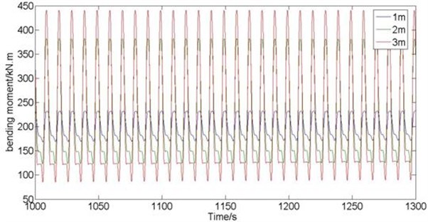
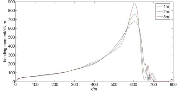
Fig. 16Comparison of distributed bending moments of riser along length direction
Under three kinds of seabeds, the dynamic displacement time-history curve of the deepest penetration node in the interval of 1000 s-1300 s was shown in Fig. 14. With the increase of the heave amplitude of the upper floating body, the penetration depth was increased obviously, the amplitude of motion was also increased significantly, and the equilibrium position was declined meanwhile.
Under different heave amplitudes of the upper floating body, the bending moment time-history curve of the deepest penetration node in the interval of 1000 s-1300 s was shown in Fig. 15. With the increase of the heave amplitude of the upper floating body, the bending moment amplitude was increased gradually, and the changing magnitude was increased significantly. The overall trends were the same under three conditions. In accordance with the method analyzed in the previous section, the maximum bending moment of the riser along the length direction was obtained in Fig. 16. It could be found from the figure that, with the increase of the heave amplitude, the bending moment of the riser movements was increased gradually, and the riser bending moment was shown in the trend of rising first, decreasing then, and reaching the maximal value at the touchdown zone.
5.3. Effect of seabed soil strength on dynamic characteristics of pipe-soil interaction
The heave amplitude of 2 m, heave cycle of 10 s, three conditions of low, middle and high soil strength were selected in the paper. And the effect of different strengths of seabed on the riser penetration depth, touchdown zone shape and bending moment was studied.
The touchdown zone shape of the riser under three seabed strengths was shown in Fig. 17. Under the same motions of the upper floating body, the riser penetration depth was declined gradually along with the increase of the seabed soil strength.
Fig. 17Touchdown zone shape of riser
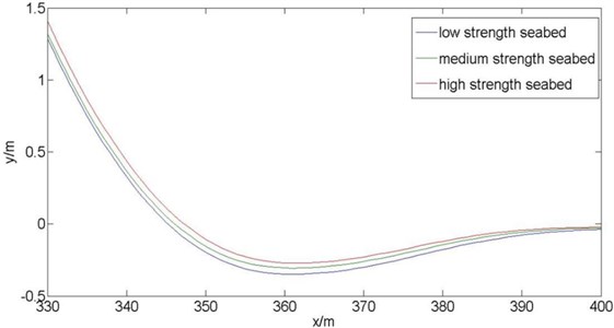
Fig. 18Time-history curve of dynamic displacement
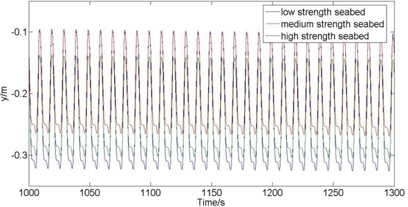
The dynamic displacement time-history curve of the deepest riser penetration point in the interval of 1000 s-1300 s was shown in Fig. 18, which was under the heave amplitude of 2 m, heave cycle of 10 s, three conditions of low, middle and high soil strength. With the increase of the seabed intensity, the amplitude of the riser penetration point was declined gradually, the penetration depth was decreased little by little, and the changing amplitude of the movement was also reduced gradually.
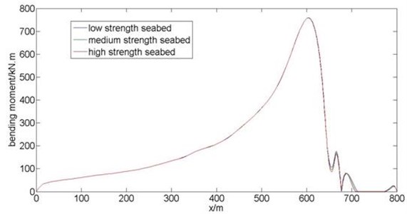
The dynamic bending moment time-history curve of the deepest riser penetration point in the interval of 1000 s-1300 s was shown in Fig. 19, which was under the same motions of the upper floating body and different seabed soil strengths. The maximal bending moment of the deepest riser penetration point was of a little change with the variation of the seabed soil strength, and the changing magnitude of the moment was increased gradually with the increase of seabed soil strength. In Fig. 20, the bending moment curve changed along the length direction was shown by means of the method described in the previous two sections. Under sea-beds with three different strengths, their riser bending moments along with the length direction were shown as the basically same trends of rising first, decreasing then, and reaching the maximal value at the touchdown area. The riser bending moment at the high- intensity touchdown zone was slightly larger than that at the low-intensity seabed with no significant difference, which was basically consistent with the result obtained in Fig. 20. Namely, the higher the intensity was, the changing amplitude of the riser bending moment would be.
Fig. 19Time-history diagram of dynamic bending moment
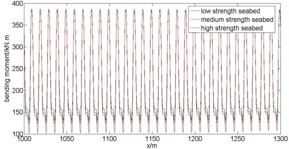
Fig. 20Comparison of riser bending moment along length direction
6. Conclusions
The nonlinear seabed with low, medium and high intensities were selected in the paper, their shear strengths were 2.8 kPa, 3.1 kPa and 3.4 kPa, and the corresponding shear strength gradients were 1.6 kPa/m, 1.8 kPa/m and 2.0 kPa/m respectively. The heave amplitude of the floating body was 1 m, 2 m and 3 m, respectively and the heave cycle was 10 s. Under different conditions, the touchdown zone shape of the riser, maximum penetration depth, dynamic time-history response of the deepest penetration point and bending moment changes were analyzed to study the impact of the seabed model, seabed strength and floating body motion on the dynamic response of the riser. And the following conclusions were obtained through the comparative analysis:
1. A dynamic characteristic model of the pipe-soil interaction was established in the paper. And experiments were conducted then to verify the numerical model. It could be seen from the result that the experiment and simulation values were close in terms of both the trend and numerical value, indicating that the numerical model was reliable, and could be used for a subsequent analysis.
2. Compared with the nonlinear seabed, the riser penetration depth at linear seabed condition was deeper, and their vertical displacement fluctuations at the deepest penetration point were of greater difference. Under both seabed conditions, the maximum bending moment at the touchdown zone was of little difference. However, the fluctuating amplitude of the bending moment under the linear seabed condition was smaller, indicating that the pipe-soil interaction simulated by the linear seabed could obtain the calculation result greater than the true value.
3. When the seabed had the same strength:
(1) As the heave amplitude of the upper floating body increased, the riser penetration depth at the touchdown area was gradually increased.
(2) As the heave amplitude of the upper floating body increased, the fluctuation range of vertical displacement at the deepest penetration point was gradually increased.
(3) As the heave amplitude of the upper floating body increased, the riser bending moment along the length direction was increased gradually. However, its overall trend was basically the same, namely, rising first, decreasing then, and reaching the maximal value at the touchdown area. The greater the heave amplitude value was, the larger the bending moment at the touchdown area would be. In addition, the changing magnitude of the cutting bending moment was increased.
4. When the floating body was in the same condition:
(1) With the increase of the seabed strength, the riser penetration depth was gradually reduced.
(2) With the increase of the seabed strength, the fluctuation range of the vertical displacement at the maximum penetration depth was gradually declined.
(3) The trends of the riser bending moment were basically same along the length direction, namely, rising first, decreasing then, and reaching the maximal value at the touchdown area. The maximum riser bending moment was slightly increased with the increase of the seabed intensity, and the fluctuation magnitude was increased significantly.
References
-
Randolph M. F., Quiggin P. Non-linear hysteretic seabed model for catenary pipeline contact. 28th International Conference on Ocean, Offshore and Arctic Engineering, OMAE, Honolulu, HI, USA, 2009.
-
Huang W. P., Meng Q. F., Bai X. L. The simulation of the interaction between SCR and seabed. Engineering Mechanics, Vol. 30, Issue 2, 2013, p. 14-18.
-
Elliott Bradley J., Zakeri Arash, MaCneill Andrew, Phillips Ryan, Clukey Edward C., LiGeorge Centrifuge modeling of steel catenary risers at towndown zone. Part II: Assessment of centrifuge test results using kaolin clay. Ocean Engineering, Vol. 60, 2013, p. 208-218.
-
Bai Y. Subsea Pipeline and Riser. 1st ed., Grenland Advanced Engineering, Inc., London, 2005.
-
Aubeny C. P., Biscontin G., Jun Zhang Seafloor Interaction with Steel Catenary Riser. Master Thesis, Texas A&M University, 2006.
-
Bridge C., Howells H., Toy N., Parke G., Woods R. Full-Scale Model Tests of a Steel Catenary Riser. WIT Press, UK, 2003, p. 107-116.
-
Theti R., Moros T. Soil interaction effect on simple-catenary riser response. Pipes and Pipeline Interaction, Vol. 46, Issue 3, 2001, p. 15-24.
-
You J., Biscontin G., Aubeny C. P. Seafloor interaction with steel catenary risers. ISOPE, Canada, 2008.
-
Jung H., Wan Y. Numerical Model for Steel Catenary Riser on Seafloor Support. Master Thesis, Texas A&M University, 2006.
-
Dunlap W., Bhohanala R., Morris D. Burial of Vertically Loaded Offshore Pipeline. OTC 6375. Houston, TX, 1990.
-
Li J. Q., He S. Q., And Ming Z. An intelligent wireless sensor networks system with multiple servers communication. International Journal of Distributed Sensor Networks, Vol. 7, 2015, p. 1-9.
-
Zhu Z., Xiao J., Li J. Q., et al. Global path planning of wheeled robots using multi-objective memetic algorithms. Integrated Computer-Aided Engineering, Vol. 22, Issue 4, 2015, p. 387-404.
-
Bridge C., Laver K., Clukey E., Evans T. Steel catenary riser touchdown point vertical action model. Offshore Technology Conference, Houston, TX, 2004.
-
Lin Q. Z., Chen J. Y. A novel micro-population immune multiobjective optimization algorithm. Computers and Operations Research, Vol. 40, Issue 6, 2013, p. 1590-1601.
-
Chen J. Y., Lin Q. Z., Hu Q. B. Application of novel clonal algorithm in multiobjective optimization. International Journal of Information Technology and Decision Making, Vol. 9, Issue 2, 2010, p. 239-266.
-
Wong K. W., Lin Q., Chen J. Error detection in arithmetic coding with artificial markers. Computers and Mathematics with Applications, Vol. 62, Issue 1, 2011, p. 359-366.
About this article

