Abstract
This paper describes design technique of solid fuel rocket motor testing system for its thrust measuring capabilities. The design process consists of 2 parts. In first part the mathematic modelling technique will be described for the mechanical section, in second – electrical. This will help to explain versatility and capabilities for coupling of the parametric design process for measurement systems design using software supported modelling tools. In order to determine the potential utility load, module design and the stability of the system in next chapter model of the system is compared with actual measurement system prototype during experimental testing and evaluation. The error between modelled and real systems is measured and discussed. The final experiment is discussed where rocket motor was tested. Modelled thrust characteristics was compared with measured data for the final discussion and conclusions.
1. Introduction
One of the major challenges in the rocket science is to maintain nominal rocket motor performance during the lift off and the rest of the flight. This concludes to problems where internal ballistics is the one of the primarily part of the equation. There are four basic key elements where one can determine the rocket motor performance characteristics: Thrust, pressure, temperature and acoustics. This paper is based on first and most important component: thrust measurements of the rocket motor. This problem employs the requirement of the analysis for the two fundamental parts in thrust measurement systems – relationship of the mechanical and electrical hardware coupling.
Many research groups which are dedicated to thrust systems design using relatively the same methods for propulsion systems thrust measurements [1, 2]. Most common thrust measuring systems is hydraulic [3], piezoelectric [4] or load cell based [2]. Hydraulic systems are losing its interest in thrust measurements because of more reliable electronic measurement systems. Most robust and versatile is load cell based measuring systems because of their capability to use the same load cell for different ranges of trust measurements. In this paper one describes a load cell with two working points for different thrust rocket motors testing.
The solid rocket motor testing stand consists of testing stand structure, thrust sensor, amplifier and analog – digital converter, recording device. The testing stand structure has to maintain rapidly changing thrust force based on direction (in this particular system setup) and at the same time to be able suppress motor displacement along – direction but let motor slide as free as possible in + direction. In other case adverse oscillations may occur [5]. This setup ensures reliable thrust measurements during experimental testing. In the next chapter the behavior of the testing stand structure will be discussed more.
The thrust measurement sensor (load cell) consists of machined metal part where strain gauge array is attached in Wheatstone bridge setup. In this particular setup four strain gauge sensors were used in pairs by active and balancing arrangement. Specifically, for this system load cell was designed for two measuring ranges: 0-10 kN and 0-15 kN. This is crucial to use suitable load cell working point where measuring range is bigger than designed maximum motor thrust because of possibility of unstable fuel grain burn and probability of thrust spikes formation which can cause damaging of the measuring system [6].
The amplifier was designed using operational amplifiers in the instrumental amplifier setup. The calculations and modeling was performed based on load cell mechanical characteristics which was derived from equations. As data recording unit one was used computer with Bruel & Kjaer “Pulse” software [7].
The aim of this paper is to propose and evaluate design methods for load cell based thrust measurement systems which can be designed parametrically with ease of capability to customize and adapt working ranges of thrust measurement for solid rocket motors.
2. Rocket motor
The rocket motor is shown in the Fig. 1 and consists of seven main parts: 1. Igniter, 2. Pressure cover, 3. Nozzle, 4. Fuel grain, 5. Grain casing and thermal protection layer, 6. O-rings and gaskets, 7. Head.
The designed characteristics of the rocket motor are described in Table 1.
Fig. 1Solid propellant rocket motor components
Table 1Solid propellant rocket motor characteristics
Properties | Values | Units |
Nominal thrust | 12000 | N |
Maximum thrust | 13000 | N |
Average thrust | 10000 | N |
Burn time | 3.5 | s |
Propellant mass | 18 | kg |
Motor mass | 33.5 | kg |
Total impulse | 33000 | Ns |
Specific impulse | 187 | s |
Rocket motor produces thrust when burned propellant escapes from throat of the rockets nozzle. It is crucial that mass flow rate Eq. (1) would be stable at all period of motor operation cycle until sliver zone is reached because otherwise the oscillations in thrust graph will occur and this could lead in burn instability and increased measurement error possibility:
where: – density of the propellant [kg/m2], – surface area of the propellant grain [m2], – burn rate [kg/s].
In this particular design the neutral star type [8] of propellant grain was used. Which means that surface area of the burning propellant is constant despite time increment until sliver is reached. To determine desired rocket motor thrust characteristics [9] it is crucial to choose right cross section geometry of the propellant grain and establish desired area of burning surface because rocket motor thrust is directly related with fuel grain area Eq. (2):
Fig. 2Propellant grain during burning

The equations below describe how thrust is produced during burn Eqs. (3), (5) and (8) of propellant and derivation of total impulse Eq. (6) and specific impulse Eq. (7) of the rocket motor:
where: – mass flow, – exit velocity, – exit pressure, – atmospheric pressure, – exit area, – thrust:
where: – gravitational acceleration the surface of the earth, – mass:
Fig. 3Modelling results of the rocket motor
After nozzle is added into system equations became:
where: – throat area, – throat pressure, – throat temperature, – specific heat ratio, – gas constant, – Mach number at nozzle exit.
The equations were employed into mathematic model using Matlab software. In Fig. 3 one can see output graph of the designed rocket motor thrust and pressure curves.
3. Load cell
Based on the modeling results the load cell was designed for working point 0.75-10 kN and working point 0.5-15 kN thrust measurement ranges. For load cell model D16T1 aluminum alloy was used 75 GPa [10]. It is recommended that working point bb should be in range of . In Fig. 4 one can see load cell geometry with parameters. It must be noted that load cell thickness parameter in this geometry is not visible. This parameter is noted as it was recommended for the load cell thickness described as .
For the diameter parameter it is recommended that should be in range of and its center e be at . For parametrization it is recommended to use values same as . Next set of equations describe the behavior of the load cell and its mechanical properties Eq. (13) where axial stress is described, Eq. (14) bending stress, Eq. (15) stress to the sensors active zone, Eq. (16) maximum stress and in Eqs. (17) and (18) bending coefficient:
where :
Fig. 4Load cell geometry
Fig. 5Load cell mechanical model geometry results graph
The strain of the load cell sensor point is calculated to check structural integrity of the whole system. Its recommended that the should be in the range of 02000e-06. It was found that best results are achieved when is approximately in 1500e-06 range. In this particular case the was 1547e-06. In Fig. 5 one shows the modelled load cell for the particular case.
To calculate the elongation of the load cell at the sensor point for the design conditions of the 10 kN and 15 kN load points Eq. (19), Eq. (20) and Eq. (21) is used. This equation helps to check if sensor of the load cell is capable to measure projected range of force. Typically, the tenzo sensor is capable to register measurements at max 1 % or 1.8° of its bend. In this particular case the bend of 0.154 % or 0.278° was reached. The sensor was SGD-7/350-DY43 [11] This data is crucial for designing robust instrumental amplifier:
4. Instrumental amplifier
Designing instrumental amplifier is crucial to calculate mechanical input data property, because one can deviate very aggressively when calibrating such system. Based on this particular case used strain gage one has found that – the bending coefficient was 2.06. This coefficient may differ if another type of strain gages are used so careful study of datasheet is recommended. For the amplifier four gages was used. Two was in active mode and two in passive for balancing purposes of the Wheatstone bridge Fig. 6.
The input voltage for the amplifier was 5 V. In Eq. (23) one is show the method for calculating the output voltage form the maximally unbalanced bridge (10 kN and 15 kN) and how many times this output must be amplified (if output voltage is 5 V) to be able registering and recording output signal Eq. (23). In this case one was found that output voltage is 0.00796 V and requirements for the amplifier are 627.455 times amplification of the input signal from the bridge:
For the sake of simplicity, instrumental amplifier was designed using same values for all operational amplifiers (Fig. 7). was selected for 10 kΩ value and was calculated based on amplifier requirements.
Fig. 6Wheatstone bridge
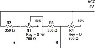
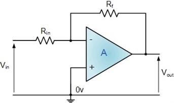
Fig. 7Operational amplifier
The first stage of amplification is done at buffer level (Fig. 8). Since and is the which are constant the is calculated using dependence of which is the quotient of the requirement of the amplification divided by product of number operational amplifiers used in the system. In this particular case the divisor for was 33 because one has used 3 operational amplifiers. So for the buffer stage was double the because 2 amplifiers in buffer stage were used. In this case was 46.478 and was 13.5 times of amplification. The values for where in this case it was noted as Eq. (24). One was found that 430 Ω:
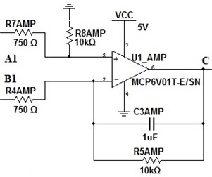
The second amplification stage (Fig. 9) have two resistors and . Because they the same it can be described as . So to find one has use Eq. (25):
Fig. 8Buffer stage of instrumental amplifier
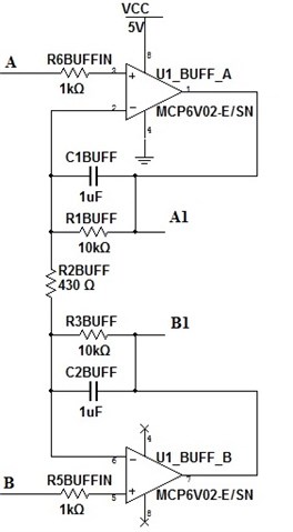
Fig. 9Amplification stage of instrumental amplifier
One must be noted that resistor values obtained from calculations not always those described can be used in reality because of resistor manufacturers using standard resistor values. In this case one must pick closest available resistor with smallest value deviation from calculated. By assessing this fact additional check is made to determine the error of the ideal and real modelled systems Eqs. (26), (27) and (28). One must be noted that and is resistor values which are closest by value to and resistor values which can be found in the market. determine the output of volts in the real model. in this case one has found that is equal to 5.048 V. Considering that is higher than power supply voltage one must be included in this surplus of voltage as error:
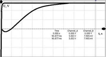
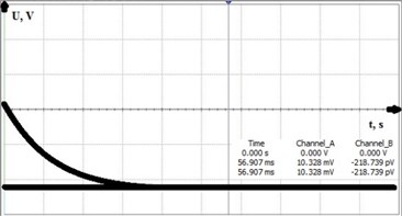
Using the model which was described above analysis was made to determine system step response and settling time. First test was performed to check systems step response. Step was set for the maximum thrust of the rocket motor which was 15 kN. In Fig. 10 one can see results of the step response. It was found that system error became minimal after 90.877 ms when ideal power supply was 5 V and fully unbalanced bridge produced 7.905 mV. for the settling case one was found that system fully settles after 56.907 ms when load cell is loaded 0 N.
Fig. 10System reaction to step response and settling time
After comparing ideal and modelled systems it was found out that amplification error was 0.149 %. Result was derived from equations below Eq. (29) and Eq. (30):
5. Experimental testing
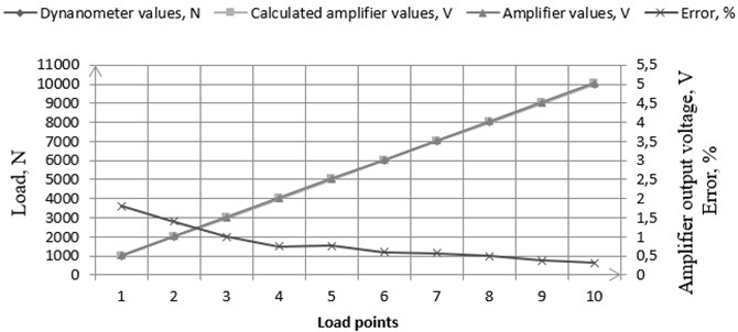
System was calibrated with high precision dynamometer where model results was compared with produced thrust measurement system based on modelling. in Fig. 11 and in Table 2 one can see calibration results where load was applied to cover whole measurement range of the load cell. It must be noted that pressing system which was used for the calibration was capable to load for maximum of 11 kN where load cell was designed for maximum 15 kN. However, load cell was designed to work at two measurement ranges which was 10 kN and 15 kN.
Table 2Calibration results
Load increment number | Dynamometer values, N | Model results, V | Real system results, V | Error, % |
1 | 1000 | 0.5 | 0.509 | 1.8 |
2 | 2000 | 1 | 1.014 | 1.4 |
3 | 3000 | 1.5 | 1.515 | 1 |
4 | 4000 | 2 | 2.015 | 0.75 |
5 | 5000 | 2.5 | 2.519 | 0.76 |
6 | 6000 | 3 | 3.018 | 0.6 |
7 | 7000 | 3.5 | 3.52 | 0.571 |
8 | 8000 | 4 | 4.02 | 0.5 |
9 | 9000 | 4.5 | 4.517 | 0.377 |
10 | 10000 | 5.003 | 5.019 | 0.319 |
By limitation of testing hardware 1 of 2 possible working points was calibrated. After calibration one was found that measuring error was relatively small and was in range from 0.319 % to 1.8 %. Assuming that this system was designed for rocket motor which average thrust is 10 kN one can consider that real error should not exceed 0.6 % in rocket burning time until sliver is reached.
Fig. 11Calibration results
Experimental testing was performed in outdoor conditions. For thrust measurements static rocket motor testing stand was used with attached load cell. Amplifier and data recording computer was used at safe distance for motor igniter initiation. Fig. 12 shows stop frame of the particular experiment.
Fig. 12Experimental testing

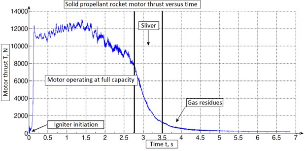
After experiment raw data was processed using Matlab software which is shown in Fig. 13 to extract only valuable information for obtaining thrust graph [12]. One has found that modelled rocket and experimental rocket motor thrust graphs deviation was as predicted. One must be noted that there were some differences from compared modelled and experimental obtained graphs. In model graph igniter produced thrust force was not included into account which enchanted deviation at very beginning after thrust curve started to buildup. From experimental data one has found out that rocket motor produced maximum thrust of 13054 N and average thrust was 10576 N before sliver. Total impulse was 32995 N∙s and specific impulse was 186.6 second.
Fig. 13Thrust graph of rocket motor during experiment
6. Conclusions
To test design requirements, rocket motor internal ballistics model was implemented with Matlab software. The maximum thrust of the modelled design was 12672 N, total impulse was 33000 N∙s and specific impulse was 187 seconds. The thrust graph from the model was used for future design steps. Mechanical parameters were selected for most suitable thrust measurements. One was found that best design for load cell working points is 10 kN and 15 kN. the bending strain of the load cell was 1547e-06 and maximum bend of strain gage was 0.154 % or 0.278°. The parametric model for mechanical geometry of the load cell was calculated and based on obtained data instrumental amplifier was designed. The theoretical model and real amplifier maximum error after comparison was 1.8 % at 1 kN load where output voltage was 0.509 V and minimum error of 0.319 % at 10 kN load where output voltage was 5.019 V. After experimental testing the measured rocket motor thrust characteristics was obtained. Maximum thrust which was produced from rocket motor was 13054 N, total impulse was 32995 N∙s and specific impulse was 186.6 seconds. The error of modelled maximum thrust and measured maximum thrust was 2.92 %. The total impulse error was 0.015 % and specific impulse error was 0.213 %. After modelled and experimental results comparison one can consider the robustness and accuracy of the design method for thrust measurement system for solid propellant rocket motor.
References
-
Desrochers M. F., Olsen G. W., Hudson M. K. A ground test rocket thrust measurement system. Journal of Pyrotechnics, Issue 14, 2001, p. 50-55.
-
De Lucena S. E., De Aquino M. G., Caporalli-Filho A. A load cell for grain-propelled ballistic rocket thrust measurement. Proceedings of the Instrumentation and Measurement Technology Conference, Vol. 3, 2005, p. 1767-1772.
-
Ren Z., Sun B., Zhang J., Qian M. The dynamic model and acceleration compensation for the thrust measurement system of attitude/orbit rocket. WMSO’08 International Workshop on Modelling and Simulation and Optimization, 2008, p. 30-33.
-
Sun B., Qian M., Zhang J. Review and prospect on research for piezoelectric sensors and dynamometers. Journal – Dalian University of Technology, Vol. 41, Issue 2, 2001, p. 127-134.
-
Mason D. R., Folkman S. L., Behring M. A. Thrust oscillations of the space shuttle solid rocket booster motor during static tests. AIAA Paper, Vol. 79, Issue 1138, 1979, p. 18-20.
-
Brownlee W. G., Marble F. E. An experimental investigation of unstable combustion in solid propellant rocket motors. ARS Progress in Astronautics and Rocketry: Solid Propellant Rocket Research, Vol. 1, 1959, p. 455-494.
-
Peterson J. S., Bartholomae R. C. Design and instrumentation of a large reverberation chamber. Proceedings on Noise-Con, 2003, p. 23-25.
-
Rafique A. F., Zeeshan Q., Kamran A., Guozhu L. A new paradigm for star grain design and optimization. Aircraft Engineering and Aerospace Technology: An International Journal, Vol. 87, Issue 5, 2015, p. 476-482.
-
Hartfield R., Jenkins R., Burkhalter J., Foster W. A review of analytical methods for solid rocket motor grain analysis. 39th Join Propulsion Conference and Exhibit, 2003, p. 1-15.
-
Korobow A. I., Batenev A. V., Brazhkin Y. A. Nonlinear elastic properties of D16 aluminum alloy and KCh35-10 cast iron. Moscow State University, Moscow, 1999, p. 106-110.
-
Gillette O. L. Measurement of static strain at 2000 °F. Experimental Mechanics, Vol. 15, Issue 8, 1975, p. 316-322.
-
Taylor T. S. Introduction to Rocket Science and Engineering. Boca Raton CRC Press Taylor and Francis Group, Philadelphia, 2009, p. 89-92.
About this article
