Abstract
A new velocity model based on dynamic cluster was proposed in this paper. During the process of iteration, the sensors can be formed a cluster according to the velocity similitude degree. Based on the assumption that the speeds from source to each sensor in the same cluster are equal, the corresponding objective function was proposed to solve the source location, which didn’t include the velocity parameter. It not only avoided the error from field measurement and the inversion, but also appropriated for the actual situation that the speeds from every source to different sensors are different. By analyzing 24 different cases, the positioning accuracy based on the velocity model proposed in this paper was verified to be preferable and stable, no matter the source is within the region of the sensor’s array or not. Even for the cases of different velocity variation ranges, the velocity model was still reliable.
1. Introduction
The technologies of MS/AE monitoring has become a very important tool in assessing the stability of a rock mass, and they have been increasingly applied in the engineering fields including mining [1], hydropower dam [2], tunnel excavation [3] and other industries after years of development. In practical rock engineering, a micro-seismic event refers to those that the majority frequencies of the induced seismic waves are within the range from 10 Hz to 103 Hz. And the accuracy level is the key point of micro-seismic monitoring, which can be achieved in estimating the event location. Generally, the location precision depends on the location method, reasonable sensors’ array configuration [4], and associated filtering and waveform identification technique [5] and so on. For the given sensors’ array, the location method is the most important factor.
According to the basic principles of micro-seismic location, there are two categories of source locating algorithms, which are the non-iterative algorithm and the iterative algorithm. The non-iterative algorithms generally include the triaxial approach [6], the zonal location method [7], INGLADA [8], the USBM algorithm [9] and so on. The former two methods are highly influenced by the geologic structure and characteristic of the rock material, while the last two methods mainly determine the source location by solve linear system of equations. When the number of sensors is less than five and the field measured data is reliable, the non-iterative algorithm can be adopted. However, when the number of sensors that collected the signal from source is bigger than five, the number of nonlinear equations will increase drastically. In such a case, it becomes difficult to accurately determine the location of the micro-seismic event using non-iterative algorithms, whereas the iterative algorithms can find the best approximation of the event location by iteration, especially for the case of low quality data measured in field or the number of sensors collected the signal from source is bigger than five.
The implementation of an iterative algorithm requires selecting a proper velocity model. According to the difference among velocity models, the existing velocity models can be divided into two kinds, single velocity model and multidirectional velocity model. The single velocity model also can be divided into two kinds based on the velocity parameters’ sources, single velocity model based on field measurement and single velocity model based on inversion. For the multidirectional velocity model, the number of unknown parameters is bigger than the number of equations if the velocity parameters determined by inversion, so there is only one kind of multidirectional velocity model, which is achieved by field measurement. The difference of models based on field measurement and inversion is that the former uses pre-measured wave propagation velocity or velocities, while the later considers the wave velocity as an unknown in the analysis. A single velocity model assumes that the wave propagation velocities to different sensors are the same, while they can be different based on the multidirectional velocity model. In fact, the stress wave propagation velocity from a micro-seismic source to different sensors may be different. All the three existing velocity models highly rely on the accuracy of the pre-measured stress wave propagation velocity at field or the applied inversion velocity. Besides, they all need an assumption that the speeds from each source to sensors are equal, which is quite different from the actual situation.
A new velocity model based on dynamic cluster was proposed in this paper. During the process of iteration, the sensors can be formed a cluster according to the velocity similitude degree. It was assumed that the speeds from source to each sensor in the same cluster are equal, and the corresponding objective function was proposed to solve the source location, which didn’t include the velocity parameter. Not only the error from field measurement and the inversion were avoided, but also the actual situation was reflected that the speeds from every source to different sensors are different. By analyzing 24 different cases, the proposed velocity model iterated by the Simplex method is found to be the best option no matter the source is within the region of the sensor’s array or not. Even for the cases of different velocity variation ranges, the positioning accuracy was still preferable.
2. Traditional velocity models in source location
2.1. Basic principles in source location
For each sensor (), assuming the stress wave propagation velocity from a MS source is (), the three dimensional coordinates of the sensor and the MS source are and respectively, is the arrival time of stress waves from the MS source to the sensor and is the origin time, it has the relation:
Assuming the calculated coordinates of the source is during the iteration process, where the origin time is , the velocity from the estimated source to the sensor is , the arrival time from the estimated source to the sensor can be calculated by:
The residual time for each sensor is then given by:
And the objective function for each coordinate of source is:
The traditional iterative algorithms aimed to minimize the objective function in Eq. (4) based on different velocity models. As the velocity from each source to different sensors can be different, three kinds of velocity models and corresponding objective functions were adopted in the past research based on different research assumptions.
2.2. Traditional velocity models
2.2.1. Single velocity model based on field measurement
Assumption: The values of velocities from MS sources to different sensors are the same, and the value obtained from the wave velocity experiment is equal to the actual propagation speed.
Assuming the velocities from a MS source to different sensors has the same value of , which is determined by field measurement near the area of the MS source, the objective function in Eq. (4) can be rewritten as:
Since there are three unknowns only in Eq. (5), at least three sensors are required to locate the MS source based on this model. The effectiveness of this model depends on the accuracy of the pre-measured velocity and the homogeneity of the rock mass.
2.2.2. Single velocity model based on inversion
Assumption: The velocities from MS sources to different sensors have the same value.
Assuming the velocities from a MS source to different sensors have the same value , which is assumed to be an additional unknown just like the coordinates of an MS source, the objective function is changed to be:
Due to that the additional known, i.e. is introduced, at least four sensors are required based on this model. The disadvantage of this model is that the rock mass is also assumed to be homogenous.
2.2.3. Multidirectional velocity model based on field measurement
Assumption: The velocities from different sources to sensor have the same value , which is determined by field measurements near the area of potential MS sources.
The objective function then becomes:
Obviously, the accuracy of this model highly relies on the field measurement of velocities which is dependent on the accuracy of the estimations of the MS sources.
Beside the objective functions given in Eq. (4) to Eq. (7), other kinds of objective functions have also been proposed [10, 11, 12, 13]. Due to space limit, details of the coupled velocity models and their corresponding objective functions will not be introduced in this paper.
3. Source location method based on dynamic cluster velocity model
3.1. Dynamic cluster method
3.1.1. Research assumption
The above three traditional velocity models all need the assumptions that the velocity value from all the sources to sensors are equal or to some single sensor are equal. In fact, because of the difference of sources, the velocity value from different sources to the same sensor are to totally different. In such case, there is a big gap between the assumption and the actual condition. For this reason, a new research assumption was proposed in this paper.
Assumption: First, all the sensors can be grouped into clusters according to their velocity similarity, and the sensors whose velocity values from some single source are similar are separated into the same cluster. Then the assumption can be proposed that the velocity values from some single source to the sensors in the same cluster are equal.
Theoretically, the new assumption has two obvious advantages comparing with the assumptions in three traditional velocity models. For one thing, it realized the expression that the velocity values from different sources to the same sensor are different, which is more reasonable. For another, the difference between the assumption and the actual condition was reduced to the minimum, because the sensors with similar velocity value were divided into the same cluster through the assessment function of velocity similitude degree. The location principle of the new method proposed in this paper is shown in Fig. 1.
Fig. 1Location principles based on new method
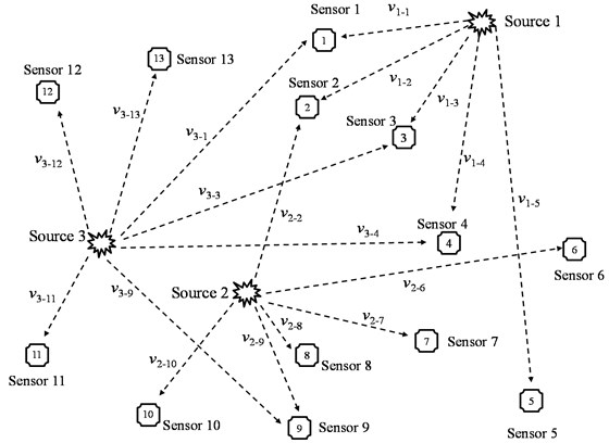
As shown in Fig. 1, for source 1, sensor 1, 2, 3, 4, 5 were gathered only because the velocities from source 1 to them were similar. In a similar way, the only reason why sensor 2, 6, 7, 8, 9, 10 were gathered into the same cluster is not which sensor is far away from source 2, but their velocities similitude degree from source 2 to them. This situation is similar from source 3 to sensor 1, 3, 4, 9, 11, 12, 13.
3.1.2. Assessment function of velocity similitude degree
According to the analysis above, it is quite important to build a suitable assessment function of velocity similitude degree and its threshold interval. In order to group the sensors with similar speed into the same cluster, the assessment function of velocity similitude degree should be built, and then the dynamic cluster can realize during the process of iteration.
When the number of sensors collected the signal from the source is , choosing , and the arrival time for each sensor is , , , , .
If , then:
Let:
When Eq. (9) is subtracted by Eq. (8), it has:
Name the value of as based on the assumption of , and then:
Similarly, the value of is , based on the assumption of :
The value of is , based on the assumption of :
For all the , , they can represent the value of based on different assumptions.
For the reason of , and it is difficult to decide whether is bigger than 0 or not, so let:
Equation (17) can be used to represent the values of under different assumptions, which is the assessment function of velocity similitude degree.
Sort in order of size, and the sensors with similar can be treated as similar speed, which can be separated into the same cluster, while the others can be excluded of the cluster.
For the case of the arrival time of some sensor is the same as , the sensor can be treated into the same cluster just as sensor 1.
The value of threshold interval, which can require the minimum number of sensors, can be treated as the initial threshold interval. After setting the threshold interval of the group, all the sensors can be initially grouped.
3.1.3. Dynamic cluster
As described above, the threshold interval should be set to complete the dynamic cluster, and the process of dynamic cluster is as follows:
1) Core cluster conduction
Theoretically, the closer distance between source and sensor, the smaller error can be obtained. So the nearest sensor can be treated as the first sensor of core cluster. And the core cluster can be conducted through two basic principles. First, the number of cluster’s sensors is bigger than four. Second, the initial threshold interval should be satisfied. The rest sensors, which were excluded of the core cluster, can be used to conduct the other clusters.
2) Dynamic correction of core cluster
The iteration can be started to solve the source location according to the method described in section 3.2. If the iteration stop requirement wasn’t satisfied, the core cluster should be corrected and the dynamic cluster can be realized. The main correct rules include: a. changing the sensors in the cluster; b. changing the threshold interval; c. including the sensors outside the core cluster into the core cluster.
3) Iteration
During the process of iteration and dynamic cluster, when the computational accuracy satisfied the stop requirement, the iteration can stop. And the stop requirement was always set as e-6. The value of objective function can be obtained when stop the iteration.
4) Optimization and checking
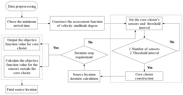
In order to avoid the iterative calculation getting into local optimum, the sensors outside the core cluster can be dealt with as the core cluster. Similarly, another value of objective function can be obtained. Optimization and checking should be done by comparing the two values of objective function, such as variance, the error of mean square and so on, and the better one is the final answer. The main flow chart of dynamic cluster and source location is as follows:
Fig. 2Flow chart of dynamic cluster and source location
3.2. Source location method based on dynamic cluster
For the sensors in the same cluster, the source location can be done according to the research assumption proposed above, the details are as follows.
For the sensor , which is in the same cluster, the wave velocities from a MS source to them are the same, , and the arrival times to them are:
Let:
When Eq. (18) is subtracted by Eq. (19), Eq. (20) … and Eq. (21) respectively, it has:
(1) If , then:
Taking the right side of the equation to the left, then:
The available data at a monitoring field include the coordinates of all the sensors and the measured arrival time to different sensors. The unknown entities are the coordinates of the MS source. In Equation (30) …and Equation (31), equations in all, a field pre-measured velocity is no longer necessary. A new objective function of which the regression value is 0 can thus been defined as follows:
The coordinates of the estimated MS source can be calculated by iterations.
(2) If (or )
Considering the assumption that the wave velocities to the three sensors have the same value, equating Eq. (18) and Eq. (19), it gives:
Reorganizing Eq. (33), it has:
Equation (34) is the middle plane equation between point and point in the three-dimensional space, and the problem of searching the MS source is then simplified into searching the source on the middle plane. And a new objective function by ignoring sensor or sensor can be adopted. When another neighbor sensor is considered, Eq. (32) can be used again as the objective function.
4. Numerical examples
4.1. Case overview
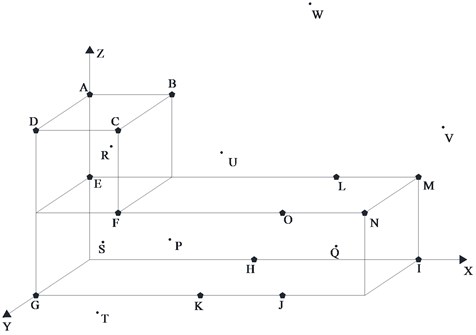
As shown in Figure 3, an example model is set to verify the effectiveness of the proposed dynamic cluster velocity model. A sensors array with fifteen sensor vertexes of A, B, C, …, N, O, four randomly selected internal sources of P, Q, R, S, three external sources T, U, V, W, are configured, and the coordinates of each point are given in Table 2 and Table 3.
Fig. 3Calculation model
In order to simulate the difference of stress wave propagation velocity in different directions, the velocity from each source to each sensor is selected by random numbers with a mean of 5 m/ms and a measurement error of 1 %, 3 % and 5 % respectively.
To choose a suitable iteration method for the velocity model proposed in this paper, Levenberg-Marquardt method (L-M method for short), the Gauss Newton iteration method (G-N method for short) and the Simplex method are adopted to solve the non-linear least squares problem of the objective function. These three methods are considered to be the most commonly used methods at present. For the convenience of expression, the single velocity model based on field measurement is abbreviated as SVFM, and the multidirectional velocity model based on field measurement is abbreviated as MVFM. Similarly, single velocity model based on inversion use SVIM for short, and the velocity model based on dynamic cluster can be abbreviated as DCVM. Compared with those using three traditional velocity models and the new model, 24 examples are set up to verify the velocity anisotropy range of 1 %, 3 % and 5 %, as listed in Table 4.
Table 2The coordinates of sensors
Sensor | X/m | Y/m | Z/m | Sensor | X/m | Y/m | Z/m |
A | 0 | 0 | 2000 | I | 4000 | 0 | 0 |
B | 1000 | 0 | 2000 | J | 3000 | 1000 | 0 |
C | 1000 | 1000 | 2000 | K | 2000 | 1000 | 0 |
D | 0 | 1000 | 2000 | L | 3000 | 0 | 1000 |
E | 0 | 0 | 1000 | M | 4000 | 0 | 1000 |
F | 1000 | 1000 | 1000 | N | 4000 | 1000 | 1000 |
G | 0 | 1000 | 0 | O | 3000 | 1000 | 1000 |
H | 2000 | 0 | 0 | – | – | – |
Table 3The coordinates of sources
Source | P | Q | R | S | T | U | V | W |
X/m | 1265 | 3329 | 603 | 356 | 907 | 1815 | 4309 | 2604 |
Y/m | 593 | 651 | 440 | 635 | 1286 | 432 | 392 | -927 |
Z/m | 487 | 379 | 1588 | 439 | –126 | 1527 | 1653 | 3328 |
Table 4Summary of location methods used in this example
Case number | Measure error range | Iterative algorithm | Velocity model | Case number | Measure error range | Iterative algorithm | Velocity model |
Case1 | 1 % | L-M method | SVFM | Case13 | 1 % | G-N method | MVFM |
Case2 | 3 % | Case14 | 3 % | ||||
Case3 | 5 % | Case15 | 5 % | ||||
Case4 | 1 % | G-N method | Case16 | 1 % | Simplex method | ||
Case5 | 3 % | Case17 | 3 % | ||||
Case6 | 5 % | Case18 | 5 % | ||||
Case7 | 1 % | Simplex method | Case19 | – | L-M method | SVIM | |
Case8 | 3 % | Case20 | G-N method | ||||
Case9 | 5 % | Case21 | Simplex method | ||||
Case10 | 1 % | L-M method | MVFM | Case22 | – | L-M method | DCVM |
Case11 | 3 % | Case23 | G-N method | ||||
Case12 | 5 % | Case24 | Simplex method |
4.2. Result analysis
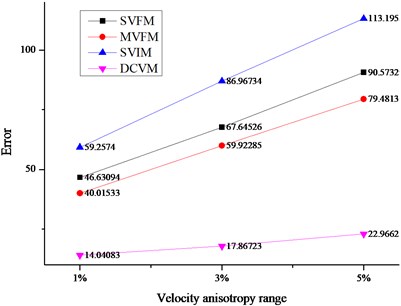
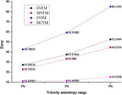
According to the difference of velocity models, the location errors were shown in Fig. 4.
As shown in Fig. 4, the disadvantages of the DCVM model are quite obvious, and the details are as follows.
(1) DCVM model appeared least affected by the change of velocity anisotropy range. As the velocity anisotropy range changed from 1 %, 3 % to 5 %, the errors based on three traditional velocity models changed dramatically. As shown in Fig. 4(a), the average errors based on SVIM model changed from 59.26 m to 86.97 m, and then turned to 113.20 m. And the rates of changing were 46.76 % and 30 % respectively. It is the similar situation with MVFM model and SVFM model. For DCVM model, the errors changed from 14.04 m to 17.87 m, and then turned to 22.97. The rates of changing were 27.28 % and 28.54 % respectively, which was obviously lower and more stable.
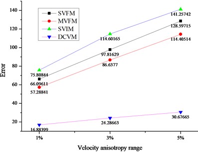
(2) The biggest advantage of DCVM model performed at the location iteration of the sources outside array. As shown in Fig. 4(b) and (c), comparing with the errors of sources inside array and sources outside array base on three traditional velocity models, the errors of sources outside array were much bigger than that of sources inside array. For the velocity model proposed in this paper, the errors were always much lower and more stable.
(3) Except for the influence of velocity anisotropy, three traditional velocity models were affected by other factors. It showed that the measure error had important influence for the two velocity models based on field measurement. Besides, the reason why the errors of SIVM model were much bigger than others is the errors produced in the process of back analysis, especially for the velocity parameters in the objective function. However, DCVM avoided the error from field measurement and the inversion.
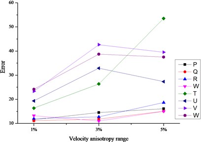
As shown in Fig. 5, through further comparative analysis on the three cases based on DCVM model, the following conclusions we can find.
(1) The errors based on DCVM model were much lower than other cases no matter which iteration method was adopted. In other words, the adoption of velocity model is much more important than the adoption of iteration method in the aspect of location error.
(2) Simplex method showed better performance than the other two methods when the velocity model is DCVM model. It was less influenced by the change of velocity anisotropy range, especially for the sources outside array.
(3) There is inconspicuous difference among location errors when the sources were solved based on DCVM model and iterated by Simplex method. In other words, the combination of DCVM and Simplex method was less influenced by the sensor array geometry. No matter the sources were within the array or not, the location errors always kept the lower level.
Above all, the effectiveness of the velocity model proposed in this paper was verified, and the combination of DCVM and Simplex method showed better performance than traditional method, which can be a better choice when the number of sensors that collected the signals from source is more than five.
Fig. 4Average location errors among different velocity models
a) Average errors for all the sources
b) Average errors for the sources outside array
c) Average errors for the sources inside array
Fig. 5The comparison charts of location errors iterated by different methods
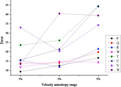
a) Location errors iterated by L-M method
b) Location errors iterated by G-N method
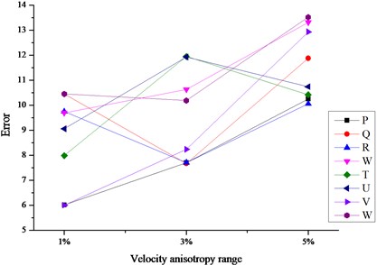
c) Location errors iterated by Simplex method
5. Discussion
The new velocity model and its corresponding objective function are easy to iterate. And during the process of iteration, all the parameters only include monitor data and three location parameters. However, users should be aware of its application conditions.
First, the minimum number of sensors is four. From an error control point of view, one should use as many sensors as possible, especially for the cases of measured data with a certain degree of uncertainties. Based on more data from sensors, the data set is statistically more reliable and generally the better array geometry will be gotten. However, the problem of source location basically belongs to the matter of solving nonlinear equations. When the number of sensors is pretty big, there will be more solutions appear. In such case, it is quite difficult to decide which one is the efficient solution, and which one is the invalid solution. When the values of velocities from source to different sensors are similar, four sensors will be enough to solve the efficient solution. And too many information, especially for the sensors with relative high degree of velocity similitude, the location error will increase obviously. And that’s the most important problem which has been solved by the velocity model proposed in this paper. Therefore, if we can’t decide whether the sensor is similar with others or not, more information of sensors needed to be collected, and the velocity model based on dynamic cluster will properly deal with all the information.
Second, the sensor array geometry needs to be optimized. Although the velocity model proposed in this paper can reduce the influence of sensor array geometry, but lots of research showed that the location accuracy was fundamentally determined by the sensor array geometry. For a certain array, the better option of location method, the higher location precision would be obtained. For the method proposed in this article, there are two basic principles, producing more planes and including more sources. The maximum number of sensors in a line is suggested to be two, which can make more planes. It will be better if the pre-evaluation of sources location was taken before the sensors were installed. In this case, the number of sources inside the sensors array geometry will be as many as possible and the sensors will get much closer to the possible sources, which can reduce the errors during the process of propagation.
Besides, for the case that the number of sensors is less than five, not only the advantages of DCVM are difficult to reach, but also the significance of iteration will lose. In this condition, some non-iterative method can be a better choice.
6. Conclusions
This paper proposed a dynamic cluster velocity model which showed obvious advantages comparing with three traditional velocity models in the field of micro-seismic sources location. The main conclusions include:
1) In order to more accurately approximate the actual situation, a new research assumption, where velocity value from source to the sensors in the same group were equal, was proposed in this paper. Based on this assumption, the process of dynamic cluster was realized according to its corresponding principles.
2) The proposed velocity model was less affected by the change of velocity anisotropy range compared with three traditional velocity models. In such condition, the influence of discrete data can reduce dramatically.
3) The combination of the proposed velocity model and Simplex method was found to be a better option to avoid the error from field measurement and inversion. Besides, the great progress was obtained for the less influence from the sensor array geometry.
References
-
Wang H., Ge M. C. Acoustic emission/microseismic source location analysis for a limestone mine exhibiting high horizontal stresses. International Journal of Rock Mechanics and Mining Sciences, Vol. 45, Issue 5, 2008, p. 720-728.
-
Xu N. W., Dai F., Liang Z. Z., et al. The dynamic evaluation of rock slope stability considering the effects of microseismic damage. Rock Mechanics and Rock Engineering, Vol. 47, Issue 2, 2014, p. 621-642.
-
Hirata A., Kameoka Y., Hirano T. Safety management based on detection of possible rock bursts by AE monitoring during tunnel excavation. Rock Mechanics and Rock Engineering, Vol. 40, Issue 6, 2007, p. 563-576.
-
Puchalski A., Komorska I. Application of vibration signal Kalman filtering to fault diagnostics of engine exhaust valve. Journal of Vibroengineering, Vol. 15, Issue 1, 2013, p. 152-158.
-
Hoshiba M. Real-Time correction of frequency-dependent site amplification factors for application to earthquake early warning. Bulletin of the Seismological Society of America, Vol. 103, Issue 6, 2013, p. 3179-3188.
-
Albright J., Pearson C. Acoustic emissions as a tool for hydraulic fracture location: experience at the Fenton hill hot dry rock site. Society of Petroleum Engineers Journal, Vol. 22, Issue 4, 1982, p. 523-530.
-
Hutton P. H., Skorpik J. R. A simplified approach to continuous AE monitoring using digital memory storage. Proceedings of Third Acoustic Emission Symposium, Vol. 16, Issue 18, 1976, p. 2-6.
-
Inglada V. The calculation of local earthquake coordinates from the few neighboring stations recorded P- or S-waves. Gerlands Beitrage zur Geophysik, Vol. 19, 1928, p. 73-98, (in German).
-
Leighton F., Blake W. Rock noise source location techniques. Taylor & Francis, Abingdon, United Kingdom, 1970.
-
Vandecar J. C., Crosson R. S. Determination of teleseismic relative phase arrival times using multi-channel cross-correlation and least squares. Bulletin of the Seismological Society of America, Vol. 80, Issue 1, 1990, p. 150-169.
-
Menke W. Using waveform similarity to constrain earthquake locations. Bulletin of the Seismological Society of America, Vol. 89, Issue 4, 1999, p. 1143-1146.
-
Li J., Gao Y. T., Xie Y. L., et al. Improvement of microseism locating based on simplex method without velocity measuring. Chinese Journal of Rock Mechanics and Engineering, Vol. 33, Issue 7, 2014, p. 1336-1346, (in Chinese).
-
Waldhauser F., Ellsworth W. L. A double-difference earthquake location algorithm: method and application to the northern Hayward fault, California. Bulletin of the Seismological Society of America, Vol. 90, Issue 6, 2000, p. 1353-1368.
About this article
This work is supported by the Award from Project of the Cheung Kong Scholars and the Development Plan of Innovative Team of China (No. IRT0950). The first author also acknowledges the support of the China Scholarship Council and the host organization the University of Western Australia for his one year visit.
