Abstract
Human activity recognition is an active research area with new datasets and new methods of solving the problem emerging every year. In this paper, we focus on evaluating the performance of both classic and less commonly known classifiers with application to three distinct human activity recognition datasets freely available in the UCI Machine Learning Repository. During the research, we placed considerable limitations on how to approach the problem. We decided to test the classifiers on raw, unprocessed data received directly from the sensors and attempt to classify it in every single time-point, thus ignoring potentially beneficial properties of the provided time-series. This approach is beneficial as it alleviates the problem of classifiers having to be fast enough to process data coming from the sensors in real-time. The results show that even under these heavy restrictions, it is possible to achieve classification accuracy of up to 98.16 %. Implicitly, the results also suggest which of the three sensor configurations is the most suitable for this particular setting of the human activity recognition problem.
1. Introduction
Human activity recognition (HAR) is one of the more recent research topics that recently gained on popularity and focus of both academic and commercial researchers. Since human activity monitoring has a broad range of applications like homecare systems, prisoner monitoring, physical therapy and rehabilitation, public security, military uses and others, the motivation to create a reliable human activity recognition system is considerable.
Generally, approaches to recognizing activities can be divided into two, usually independent, groups – sensor-based and vision-based. Sensor-based systems use various sensors that are attached to the subject being monitored. Vision-based activity recognition systems, on the other hand, try to eliminate the need for sensors and attempt to recognize subject's behavior from images and video sequences. Both approaches have their challenges arising from their nature. While sensor-based systems require classification algorithms to be as speedy as possible in order to be implemented in low-power wearable devices, accurate and reliable vision-based systems are still a challenge no matter the computation power. This paper focuses on three distinct sensor-based systems, each of which was used to create a different HAR dataset. A short description of the datasets is provided in section 2.
More often than not, time complexity of a classification algorithm is a limiting issue. While developing new methods and optimizing the existing ones is certainly the correct way of approaching the problem, it may not always be the most feasible as in some signal processing problems it may prove difficult to classify the data as fast as it is acquired. This is usually necessary because the signal is then processed as a time-series and as such needs to be as continuous as possible. In this paper, we attempt to alleviate this problem and focus on the possibility of recognizing human activities from single time points (records) given only raw, unprocessed data from the sensors. Should this approach prove possible and even reliable, the classifiers would no longer place limits on the operating frequencies of the sensors, simply discarding records when the classifier is not ready to process them without the risk of losing vital information.
1.1. Current approaches in activity recognition
In general, in activity recognition authors attempt to recognize static states (lying, sitting, standing, etc.), dynamic states (walking, running, etc.) and/or transition states (i.e. standing to walking). Data preprocessing to improve the classification accuracy is common [1-3]. Classification methods currently widely used in the area are based both on classic algorithms like the Classification And Regression Tree (CART) [4, 5] or k-Nearest Neighbor (k-NN) [6, 7] and more advanced techniques like the Adaptive Neuro Fuzzy Interference System (ANFIS) [8, 9] or Iterative Dichotomiser 3 (ID3) [10] and others.
2. Datasets
The datasets used in this paper have been acquired from the UCI Machine Learning Repository where they are freely available to download along with their description and related research papers. The goal of this paper is to learn if human activities can be reliably recognized from single time points rather than time series of a signal generated by the sensor systems without any prior preprocessing. These conditions were met by three HAR datasets available in the UCI repository: Physical Activity Monitoring for Aging People 2, OPPORTUNITY Activity Recognition Data Set and Localization Data for Person Activity Data Set, shortened in the following text as the PAMAP2, Opportunity and Localization datasets, respectively.
As each of the dataset is focused on a different set of activities, it was necessary to unify them in order to make them usable in a direct comparison. For this reason, the performed activities were grouped up into 4 classes: walking, sitting and lying with the rest of the activities being merged into the others class. The practical justification for this division lies in the fact that these three activities are the very base for any other activity, thus their reliable recognition can be considered crucial in order to be able to classify finer ones. The number of records for each class and each dataset is listed in Table 1.
Table 1The number of records per class and dataset
Activity | Dataset | ||
Localization | PAMAP2 | Opportunity | |
Walking | 32710 | 229709 | 72661 |
Sitting | 27244 | 184645 | 48041 |
Lying | 54480 | 192290 | 7044 |
Others | 50426 | 1314787 | 187689 |
Total | 164860 | 1921431 | 315435 |
Due to the different nature of each of the used sensor systems, every dataset contains parameters that the other two datasets do not. These parameters were removed, leaving the datasets with only location and movement related sensor values. Time points (records) containing any number of NaN values were considered faulty and as such were discarded. Most often, NaN values are the result of a connection loss between the sensors and the recording unit. While these records may not be completely irrelevant, they are not frequent enough in either of the datasets to have a measurable impact on classification performance if removed.
2.1. The opportunity dataset
This dataset has been created to provide a benchmark for HAR methods. It consists of three different sensor systems (wearable, ambient, object-attached) and contains a wide variety of activities described and distinguished by many parameters (sensor data, limb used to perform them, etc.). The dataset provides a total of 242 parameters, 144 of which are data from wearable sensors, that is 7 inertial record units (IMUs), 12 3D acceleration sensors and 4 3D localization sensors, 60 parameters are taken from object sensors placed on 12 objects and 37 parameters correspond to data obtained from ambient sensors (13 switches and 8 3D acceleration sensors). The dataset was collected from 4 subjects in 6 runs, during 5 of which they were performing activities of daily living (ADL) and one run was a “drill” run in which the subjects specifically performed a particular activity.
For the purposes of this paper, only the wearable sensor portion of the dataset was extracted. ADL and drill activities were merged into a single set as their division was not relevant in the task ahead. As some of the parameters were statistics computed from the records, these parameters were not taken into consideration. Overall, 133 parameters per record were used, making this dataset the most elaborate (and the most computationally expensive) of the three. Its detailed descriptions can be found in [11] and [12] with further reading on its application in, for example, [13].
2.2. The PAMAP2 dataset
The PAMAP2 dataset contains data of nine healthy human subjects, each wearing three IMUs by Trivisio, Germany and a heart rate monitor. Each of the three IMUs measures temperature and 3D data from an accelerometer, gyroscope and magnetometer. The data is sampled at 100 Hz and transmitted to PC via a 2.4 GHz wireless network. Subjects wore one IMU on the dominant wrist, one on the dominant ankle and one on the chest. Detailed information on the dataset can be found in [14] and [15].
The methods have been tested on all 9 test subjects in the dataset, labeled in the dataset as subject101 through subject109. Data of all these subjects consists of 2872532 records, each containing 54 values. The description of the values is also included in the dataset documentation. Some values can be missing, indicated with a NaN (Not a Number) value.
Aside from the total of twelve activities performed by the subjects, the dataset also contains transition activities (data collected while not clearly performing any of the desired activities). These were discarded as their relevance is not assured. Since some records contain only NaN values, these were discarded as well. From each record, irrelevant values, that is the orientation of each IMU and timestamp, were removed. Since most heart-rate values were NaNs due to a different operating frequency, they were also removed. As a result, each record contains 36 values.
2.3. The localization dataset
A simple yet very interesting dataset consisting of 4 localization tags placed on the ankles, belt and chest of the user. Originally described and used in [16], this dataset was primarily focused on detecting activities that could help identify emergency situations and provide a basis for remote care systems for elderly people. The dataset could be considered quite minimalistic as each record contains only 8 parameters: sequence ID, tag ID, timestamp, date, 3 localization coordinates for a tag and a class label. Disregarding the sequence IDs, timestamps and dates as irrelevant and separating the class label, the final dataset was the smallest one with only 4 parameters per record.
Unfortunately this dataset did not contain a pure standing activity, which is why this particular activity, while being one of the base activities for any other one, was included in the others class even though the previous two datasets do distinguish it.
3. Classifiers being evaluated
To provide an overview of learning algorithms with application to human activity recognition, nine distinct classifiers were tested, including the above mentioned k-NN and CART. Also, the OMP classifier as defined in [17] was evaluated against our own custom modification that significantly improves the reliability of the recognition. Other classifiers are Linear Discriminant Analysis (LDA) [18, 19], Quadratic Discriminant Analysis (QDA) [20, 21], Random Forest (RF) [22, 23] and Nearest Centroid Classifier (NCC) [24, 25]. The following subsections provide a brief informal description for each of the classifiers except for OMP which is described more elaborately in its own section.
3.1. k-Nearest Neighbors
k-NN is a non-parametric algorithm, meaning that it makes no assumptions about the structure or distribution of the underlying data, thus being suitable for real-world problems that usually do not follow the theoretical models exactly. The method is also considered to be a lazy learning algorithm as it performs little to no training during computation. As a result, the method uses the whole training dataset during classification. k-NN is well known for its simplicity, speed and generally good classification results in applications like bioinformatics [26], image processing [27], audio processing [28] and many others.
3.2. Classification and regression tree
This algorithm classifies a sample according to groups of other samples with similar properties. During training, the training data is continuously divided into smaller subsets (tree nodes). When the divisions are finished, the samples are clustered together according to their properties. Testing samples are then evaluated against certain conditions in each node and propagated throughout the tree. When the sample reaches a leaf node, it is then assigned the class to which the samples in that node belong. In this paper, a binary tree with logical conditions was used. CARTs are still under extensive research and can be used as a standalone classifier [29] or as a part of larger algorithmic structures [30].
3.3. Random forest
RF is an ensemble algorithm consisting of a number of CARTs combined together into a single voting system. Each CART receives a dataset with only a subset of parameters, giving it a perspective and knowledge about the problem unique from any other CART. These parameters are chosen randomly, but each parameter set is unique. The number of parameters to choose for each CART as well as the number of CARTs in the forest are the only two variables that are subjects to change when performing experiments, making it easy to use. Its downside is both time and spatial complexity inherent to its nature. However, the algorithm has been shown to be very robust in performance in many research areas [31, 32], making it a suitable alternative for consideration in both classification and regression problems.
3.4. Linear discriminant analysis
LDA is a well-known technique used to identify sample clusters in a given set of data. It attempts to divide clusters (data classes) with a linear function so that the classes are as distant from each other as possible, but at the same time keeping the distance between individual data samples in a single class minimal. The method assumes that the data in each class is normally distributed, but it has still been successfully applied in many problems of automatic recognition, for example in image feature extraction [33] or speech recognition [34].
3.5. Quadratic discriminant analysis
As the name suggests, QDA is very closely related to LDA with the exception that QDA does not assume the normal distribution of the data in each class. Instead of the linear function that separates the classes from each other, the function used by QDA is quadratic and can be considered to be a generalization of LDA. Due to its greater time complexity, the method is not as widely used as LDA, but it is still feasible in many applications, including bioinformatics [35] or molecular physics [36].
3.6. Nearest centroid classifier
An extremely fast classifier. The approach is similar to that of k-NN, but instead of k closest training samples the method picks the label of the class whose training samples' mean (centroid) is the closest to the signal query. The speed and simplicity of the algorithm is compensated by low classification performance. Therefore the classifier is usually coupled with one or more data preprocessing techniques. In many implementations the method has been successfully used to create pattern recognition systems in bioinformatics [37, 38].
4. Orthogonal matching pursuit
Well described in [39], OMP is an iterative sparse approximation algorithm that reduces data into a given number of sparse coefficients and thus can be considered a dimensionality reduction method. Given an overcomplete dictionary of observations (records), for each observation to be classified, OMP picks a number of the best fitting observations from the dictionary and uses them to compute the sparse coefficients. Those are then checked against the dictionary itself for similarity and classified.
The dictionary can be represented as an m×n real-valued matrix A, where m is the length of an observation and n is the number of observations in the dictionary (training observations). The iterative nature of the algorithm allows for sparse coefficient number to be chosen in advance. It stands to reason to limit the number of sparse coefficients s such that s≤m, although the number can be truly limited only by the number of training observations, n.
Originally, the classifier proposed in [17] requires n=t×c, where t is the number of training observations for a given class and c is the number of classes. The classification algorithm requires the training set to contain the same number of training observations for each class. It is also necessary to keep the observations of a given class grouped together. Therefore, the training matrix has the form of A=[a11,a21,…,at1,a12,…,atc], where aij, i=1,...,t, j=1,...,c is the ith training observation of class j and length m.
The proposed modification changes the meaning of t and the resulting number of observations in the training set. Here:
where is a -dimensional vector consisting of the numbers of training observations for a given class. By this, the limitation imposed on the number of training observations in the original classification approach is lifted. The sparse coefficients are obtained by finding the sparse solution to the equation:
where is the query vector, is the training matrix and is the sparse coefficient vector. The stopping criterion in the implementation is reaching the sparse coefficient vector with the desired number of non-zero values.
4.1. Classification
To classify the query signal vector, a strategy of computing the residual value from the difference between the query vector and its sparse representation converted into the vector space of the training matrix vectors is employed. This is performed for each class resulting in residuals. The classification is then based on the minimum residual. Formally, the classification problem can be stated as follows:
Here, is an -dimensional vector with non-zero elements located only on the indices corresponding to the th class in the training matrix, hence the need for the training samples of a given class to be grouped together in the matrix. The algorithm could be described by the following steps:
⦁ Set the iteration variable to 1.
⦁ Replace all sparse coefficients with indices not corresponding to class with zeros.
⦁ Multiply the training matrix with the modified vector
⦁ Compute the -norm of the resulting vector.
⦁ Increase by 1 and repeat for all classes.
⦁ Output the class whose -norm is the lowest.
Computing the residuals is generally not computationally expensive and can be performed in real time, depending on the size of the training matrix. Only very large training matrices can slow the process down significantly.
Aside from the modification above, we also used a tensor adaptation that we developed and described in [40]. This adaptation restructures the data into a tensor and implements elements of the ensemble paradigm into its classification procedure. Experiments confirming its ability to generally perform better than the original OMP version in a HAR problem was included in [40].
5. Experiments
The following section describes the workflow used to evaluate the performance of the classifiers as well as the evaluation process and its results.
5.1. Experimental settings
The execution of some of the algorithms can be customized through execution parameters which, for these experiments, were set according to the best empirical speed/accuracy ratio. While the goal was to make the results as comparable as possible despite using datasets with greatly dissimilar properties, the Localization dataset contained so few parameters that the evaluation required a different setting. The common settings in terms of customizable algorithms for all dataset were as follows: as all algorithms were implemented in the latest version of MATLAB, the default MATLAB settings were used for CART. k-NN was experimented upon with four settings of the parameter: 1, 3, 5 and 10. As k-NN is a classic and very well known classifier, we decided to include these four most successful settings as opposed to just picking one that performed the best. LDA, QDA and NCC were not customizable.
For the OMP classifiers (designated as OMP for the original version, OMPmod for the modification described in section 4 and OMPten for the tensor adapation) and RF, the number of parameters per record in the Localization dataset was limiting. While for the PAMAP2 and Opportunity datasets the methods were set to 10 sparse coefficients (OMPs) and 1000 trees each accepting 6 input parameter each (RF), the Localization dataset, due to it having only 4 parameters per record, had to make do with 2 sparse coefficients and 6 trees calculating 2 parameters each. While this setting does seem quite restrictive, OMP should compute only as many sparse coefficients as there are parameters and RF used the highest setting possible as there are no more than 6 combinations of 4 parameters taken 2 at a time.
Given the difference in the number of records in each dataset, a compromise had to be made in this area as well. The lowest number of records were in the Localization dataset (164850 records), the number of samples taken for one experiment was, therefore, reduced to 150000. As most of the samples in the other two datasets would be discarded, we performed a total of 5 completely random selections of 150000 samples. For each selection, the experiments were conducted and the results averaged, taking much greater data space of the datasets into consideration during the experiments.
The entire dataset was divided into a training and a testing set. Experiments were performed on 5 different settings with the training set being a 10 %, 20 %, 30 %, 40 % or 50 % portion of the selected samples. The rest was used for evaluation. Since not all of the classifiers provide a validation step, the step was omitted from the evaluation process. This could also be considered a kind of a restriction as it is common in data processing to use portions of about 70 % for training. Since the time complexity of the algorithms vary greatly, performance records in speed of computation time were also conducted. The times were calculated as the worst case scenario for the 50 % training set only. Note that if the classifier first created a model from the training set and then used it for classification (like CART and RF), the training part is not included as, in practice, training is usually not a time-critical computation and is done in advance. In cases when the testing phase was too fast to measure on the per-record basis (like all CART evaluations), the whole testing phase was measured and TPM (Time Per Record) was calculated by dividing the resulting time by the number of records in the test phase.
The experiments were run on a computer equipped with a quad-core Intel Core i5-750 2.67 GHz processor, 8 GB of DDR3 RAM effectively clocked at 1333 MHz, Windows 8.1 operating system and the latest version of MATLAB.
5.2. Results
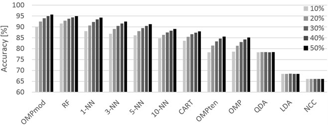
The averaged classification accuracies given as percentual success rates are shown in Tables 2-4 where the classifiers are sorted according to their best results (regardless of the training set size) in the descending order. For all methods except for LDA, QDA and NCC, larger training set resulted in more or less improved accuracy. LDA, QDA and NCC, on the other hand, suggest that in HAR problems, the training set size does not matter to them. This does not come as a surprise as no matter the training set size, data distribution (for LDA and QDA) and the centroid location (for NCC) remain the same. This property can clearly be seen in Figures 1-3 where the accuracy changes very little with the training set size. While the charts can seem rather redundant, the behavior of the classifiers is worth noticing as they all scaled about the same in terms of improving the accuracy with greater training size. Considering the variety of data acquisition devices used in the three datasets and of the classifiers themselves, the charts suggest a hidden property of the HAR problem that is certainly worth investigating. Note that in Figure 3, even though the differences between training set sizes are slightly exaggerated by a different -axis scale, LDA, QDA and NCC still show little to no difference in performance.
Fig. 1Graphical representation of the accuracies achieved for different training sets (10 % through 50 %, left-to-right order) and classifiers. Localization dataset
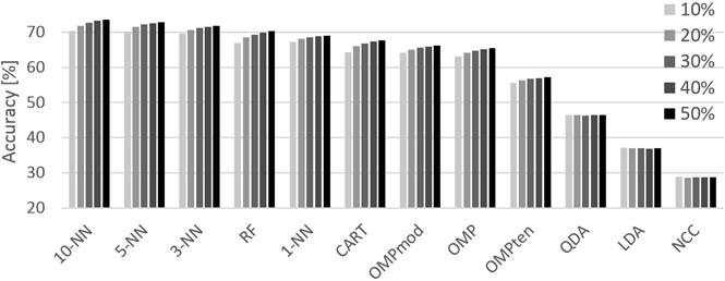
Fig. 2Graphical representation of the accuracies achieved for different training sets (10 % through 50 %, left-to-right order) and classifiers. PAMAP2 dataset
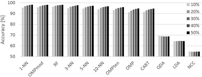
Fig. 3Graphical representation of the accuracies achieved for different training sets (10 % through 50 %, left-to-right order) and classifiers. Opportunity dataset
For the Localization dataset (Table 2), the results are generally discouragingly low, topping at 73.55 % for k-NN with . This suggests that while the dataset can provide some accuracy, the data collection setting using only four localization tags is not suitable for the task as specified in this paper. K-NN was, in this case, the best performing algorithm almost regardless of its setting. The differences between individual algorithms are not too great, giving the potential user freedom in choosing a method in terms of calculation speed.
The PAMAP2 dataset (Table 3) has shown promising results before, and the results were confirmed in these experiments as well. With the maximum accuracy at 98.16 % by 1-NN followed very closely with the difference of only 0.04 % by our proposed method, the dataset appears to present a highly reasonable compromise between accuracy and price of the data capturing solution. With the exception of LDA, QDA and NCC, the classifiers performed quite well, offering a variety of methods for solving HAR problems using the capturing settings as defined in the PAMAP2 dataset documentation.
Finally, the Opportunity dataset (Table 4) shows promising and satisfactory results while its setting seems to be the most suitable for our modification of the OMP based classifier. The classifier surpassed all other classifiers with the lead of 0.78 %, 1.45 % and 7.75 % against RF, 1-NN and CART, respectively. Practical usefulness of OMPmod over RF depends on future time complexity reduction as the method is noticeably slower than RF. It is also noteworthy that RF performed better than any other classifier for 10 % and 20 % training set sizes in PAMAP2 as well as Opportunity, however practical application with the provided accuracy results could be doubted given the potential when using more data for training.
Table 2Averaged recognition accuracy for each of the classifier per dataset size (Localization)
Classifier | Training set size | TPS (ms) | ||||
10 % | 20 % | 30 % | 40 % | 50 % | ||
10-NN | 70.36 | 71.89 | 72.72 | 73.26 | 73.55 | 6.669 |
5-NN | 70.28 | 71.53 | 72.22 | 72.64 | 72.93 | 6.059 |
3-NN | 69.58 | 70.64 | 71.23 | 71.58 | 71.90 | 5.784 |
RF | 67.01 | 68.57 | 69.35 | 69.92 | 70.30 | 8.276e-3 |
1-NN | 67.23 | 68.08 | 68.54 | 68.82 | 69.03 | 5.901 |
CART | 64.28 | 66.02 | 66.75 | 67.35 | 67.76 | 8.883e-4 |
OMPmod | 64.17 | 65.10 | 65.62 | 65.95 | 66.21 | 9.597 |
OMP | 63.18 | 64.22 | 64.82 | 65.17 | 65.43 | 6.495 |
OMPten | 55.61 | 56.40 | 56.75 | 56.97 | 57.27 | 8.427 |
QDA | 46.50 | 46.39 | 46.37 | 46.45 | 46.45 | 5.547e-4 |
LDA | 37.12 | 36.96 | 36.95 | 36.90 | 36.99 | 5.125e-4 |
NCC | 28.92 | 28.55 | 28.76 | 28.72 | 28.77 | 2.829e-4 |
Table 3Averaged recognition accuracy for each of the classifier per dataset size (PAMAP2)
Classifier | Training set size | TPM (ms) | ||||
10 % | 20 % | 30 % | 40 % | 50 % | ||
1-NN | 95.49 | 96.78 | 97.41 | 97.91 | 98.16 | 13.737 |
OMPmod | 95.80 | 96.89 | 97.46 | 97.89 | 98.12 | 200.040 |
RF | 96.28 | 97.24 | 97.61 | 97.86 | 98.05 | 1.320 |
3-NN | 94.94 | 96.21 | 96.86 | 97.33 | 97.65 | 13.748 |
5-NN | 94.55 | 95.84 | 96.49 | 96.93 | 97.25 | 13.212 |
10-NN | 93.98 | 95.34 | 95.98 | 96.44 | 96.75 | 13.631 |
OMPten | 93.15 | 94.47 | 95.12 | 95.53 | 95.91 | 123.903 |
OMP | 91.15 | 92.75 | 93.66 | 94.29 | 94.67 | 80.547 |
CART | 91.52 | 93.00 | 93.66 | 94.16 | 94.58 | 7.228e-4 |
QDA | 69.34 | 68.87 | 68.75 | 68.70 | 68.80 | 2.332e-3 |
LDA | 64.32 | 64.40 | 64.52 | 64.49 | 64.47 | 2.407e-3 |
NCC | 54.76 | 54.55 | 54.57 | 54.60 | 54.61 | 1.378e-3 |
Table 4Averaged recognition accuracy for each of the classifier per dataset size (Opportunity)
Classifier | Training set size | TPM (ms) | ||||
10 % | 20 % | 30 % | 40 % | 50 % | ||
OMPmod | 89.98 | 92.51 | 93.95 | 94.96 | 95.71 | 604.396 |
RF | 91.53 | 92.85 | 93.73 | 94.41 | 94.93 | 2.235 |
1-NN | 88.10 | 90.66 | 92.27 | 93.44 | 94.29 | 36.047 |
3-NN | 86.83 | 89.04 | 90.49 | 91.59 | 92.51 | 37.488 |
5-NN | 86.13 | 88.10 | 89.43 | 90.44 | 91.25 | 36.592 |
10-NN | 84.73 | 86.37 | 87.44 | 88.30 | 89.03 | 51.847 |
CART | 83.63 | 85.45 | 86.65 | 87.37 | 87.96 | 9.775e-4 |
OMPten | 78.33 | 81.45 | 83.36 | 84.68 | 85.58 | 82.948 |
OMP | 78.60 | 81.36 | 83.05 | 84.28 | 85.13 | 55.745 |
QDA | 78.36 | 78.45 | 78.40 | 78.37 | 78.41 | 7.826 |
LDA | 68.45 | 68.48 | 68.51 | 68.46 | 68.42 | 7.891 |
NCC | 66.11 | 66.11 | 66.12 | 66.10 | 66.09 | 5.301 |
The approximate times required to classify one record for each classifier are listed in each table in the TPM column. The values are in milliseconds. As is often the case, the least accurate ones are the fastest. This holds true in these experiments as well when the fastest of the tested algorithms, NCC, performed very poorly. QDA performed significantly better while being only slightly slower, but still could not provide satisfactory accuracy. While RF, k-NN and OMPmod are relatively slow methods in comparison, their speed is still sufficient for practical application providing, at worst, 5 classifications every second for the PAMAP2 dataset. Though the most accurate when dealing with the Opportunity dataset, OMPmod was also the slowest, providing only one to two classifications every second. In this case, practical use might depend on the requirements of the customer, but it is reasonable to assume that humans will not switch activities every second or even more often.
6. Conclusion
This paper evaluated several classification techniques and presented their success rates in human activity recognition from single time points and without any prior preprocessing. Given the sensor technology that was used to create the PAMAP2 dataset, it was shown that basic activities (walking, lying and sitting) can be recognized reliably and very precisely. Two more datasets with different sensor settings were compared with lesser accuracy results. While for the Opportunity dataset the methods performed only slightly worse, the Localization dataset has proven unsuitable for the defined task. The approach to the HAR problem proposed in this paper suggests that using the right sensor setting, problems with the follow-up classifier's time complexity can be greatly alleviated. The proposed modification of the OMP based classifier has shown excellent results for two of the datasets, but the modification's increased performance comes at the price of significantly higher time complexity. The fastest of the algorithms was NCC, but its recognition accuracy is not sufficient for practical use. From the speed/accuracy ratio perspective, k-NN and RF seem to be the most reasonable choice as their accuracy performance is surpassed by OMPmod only closely, but they have a significant edge in computation times. However, future work may prove that OMPmod can be solved in a much more time-efficient way, which will also be the focus of further research.
References
-
Khan A. M., Lee Y.-K., Lee S. Y., Kim T.-S. A triaxial accelerometer-based physical-activity recognition via augmented-signal features and a hierarchical recognizer. IEEE Transactions on Information Technology in Biomedicine, Vol. 14, Issue 5, 2010, p. 1100-1172.
-
Kim E., Helal S., Cook D. Human activity recognition and pattern discovery. IEEE Pervasive Computing, Vol. 9, Issue 1, 2010, p. 48-53.
-
Anguita D., Ghio A., Oneto L., Parra X., Reyes-Ortiz J. L. Human activity recognition on smartphones using a multiclass hardware-friendly support vector machine. In Proceedings of the 4th international conference on Ambient Assisted Living and Home Care, IWAAL’1, Springer-Verlag, 2012, p. 216-223.
-
Loh W.-Y. Classification and regression trees. Wiley Interdisciplinary Reviews: Data Mining and Knowledge Discovery, Vol. 1, Issue 1, 2011, p. 14-23.
-
Ripley B. Classification and regression trees. R package version, 2005.
-
Jatoba L. C., Grossmann U., Kunze C., Ottenbacher J., Stork W. Context-aware mobile health monitoring: evaluation of different pattern recognition methods for classification of physical activity. IEEE 30th Annual International Conference in Engineering in Medicine and Biology Society, 2008, p. 5250-5253.
-
Maurer U., Smailagic A., Siewiorek D. P., Deisher M. Activity recognition and monitoring using multiple sensor on different body positions. IEEE Internation Workshop on Wearable and Implantable Body Sensor Networks, 2006.
-
Jang J.-S. R., Sun C.-T. Neuro-fuzzy and soft computing: a computational approach to learning and machine intelligence. Prentice-Hall, Inc., Upper Saddle River, NJ, USA, 1997.
-
Ziaeefard M., Ebrahimnezhad H. Human action recognition by ransac based salient features of skeleton history image using anfis. 6th Iranian on Machine Vision and Image Processing, p. 1-5, 2010.
-
Lavanya D., Rani K. U. Performance evaluation of decision tree classifiers on medical datasets. International Journal of Computer Applications, Vol. 26, Issue 4, 2011, p. 1-4.
-
Roggen D., Calatroni A., Rossi M., Holeczek T., Forster K., et al. Collecting complex activity datasets in highly rich networked sensor environments. Seventh International Conference on Networked Sensing Systems, 2010, p. 233-240.
-
Chavarriaga R., Sagha H., Calatroni A., Digumarti S. T., Trster G., et al. The opportunity challenge: a benchamr database for on-body sensor-based acitivity recognition. Pattern Recognition Letters, Vol. 34, Issue 15, 2013, p. 2033-2042.
-
Plötz T., Hammerla N. Y., Olivier P. Feature learning for activity recognition in ubiquitous computing. Proceeding of the Twenty-Second International Join Conference on Artificial Intelligence, Vol. 2, 2011, p. 1729-1734.
-
Reiss A., Stricker D. Creating and benchmarking a new dataset for physical activity monitoring. The 5th Workshop on Affect and Behavior Related Assistance, 2012.
-
Reiss A., Stricker D. Introducing a new benchmarked dataset for activity monitoring. The 16th IEEE International Symposium on Wearable Computers, 2012.
-
Kalua B., Mirchevska V., Dovgan E., Lutrek M., Gams M. An agent-based approach to care in independent living. Ambient Intelligence on Computer Science, Vol. 6439, 2010, p. 177-186.
-
Wright. J, Yang A. Y., Ganesh A., Sastry S. S., Ma Y. Robust face recognition via sparse representation. IEEE Transactions on Pattern Analysis and Machine Intelligence, Vol. 31, 2009, p. 210-227.
-
Zhong F., Zhang J. Linear discriminant analysis based on l1-norm maximization. IEEE Transactions on Image Processing, Vol. 22, Issue 8, 2013, p. 3018-3027.
-
Mika S., Ratsch G., Weston J., Scholkopf B., Mullers K. R. Fisher discriminant anylsis with kernels. IEEE Signal Processing Society Workshop on Neural Networks for Signal Processing IX, 1999, p. 41-48.
-
Srivastava S., Gupta M. R., Frigyik B. A. Bayesian quadratic discriminant analysis. Journal of Machine Learning Research, Vol. 8, 2007, p. 1277-1305.
-
Kon M. A., Nikolaev N. Empirical normalization for quadratic discriminant analysis and classifying cancer subtypes. Fourth International Conference on Machine Learning and Applications, Vol. 2, 2011, p. 374-379.
-
Breiman L. Random forests. Machine learning, Vol. 45, Issue 1, 2001, p. 5-32.
-
Díaz-Uriarte R., Andres S. A. D. Gene selection and classification of microarray data using random forest. BMC bioinformatics, Vol. 7, Issue 1, 2006.
-
Dabney A. R, Storey J. D. Optimality driven nearest centroid classification from genomic data. PLoS ONE, Vol. 2, Issue 10, 2007, p. e1002.
-
Hastie T., Tibshirani R. Discriminant adaptive nearest neighbor classification. IEEE Transactions on Pattern Analysis and Machine Intelligence, Vol. 18, Issue 6, 1996, p. 607-616.
-
Horton P., Nakai K. Better prediction of protein cellular localization sites with the k nearest neighbors classifier. International Society for Computational Biology, Vol. 5, 1997, p. 147-152.
-
Haralick R. M., Shanmugam K., Dinstein I. H. Textural features for image classification. IEEE Transactions on Systems, Man and Cybernetics, Vol. SMC-3, Issue 6, 1973, p. 610-621.
-
Fujinaga I., MacMillan K. Realtime recognition of orchestral instruments. In Proceedings of the international computer music conference, Vol. 141, 2000, p. 143.
-
Hess K. R, Abbruzzese M. C., Lenzi R., Raber M. N., Abbruzzese J. L. Classification and regression tree analysis of 1000 consecutive patients with unknown primary carcinoma. Clinical Cancer Research, Vol. 5, Issue 11, 1999, p. 3403-3410.
-
Liaw A., Wiener M. Classification and regression by random forest. R news, Vol. 2, Issue 3, 2002, p. 18-22.
-
Zhang Q.-Y., Sousa J. A. Random forest prediction of mutagenicity from empirical physicochemical descriptors. Journal of Chemical Information and Modeling, Vol. 47, Issue 1, 2007, p. 1-8.
-
Svetnik V., Liaw A., Tong C., Culberson J. C., Sheridan R. P., et al. Random forest: a classification and regression tool for compound classification and qsar modeling. Journal of Chemical Information and Computer Sciences, Vol. 43, Issue 6, 2003, p. 1947-1958.
-
Li M., Yuan B. 2d-lda: a statistical linear discriminant analysis for image matrix. Pattern Recognition Letters, Vol. 26, Issue 5, 2005, p. 527-532.
-
Haeb-Umbach R., Ney H. Linear discriminant analysis for improved large vocabulary continuous speech recognition. IEEE International Conference on Acoustics, Speech and Signal Processing, Vol. 1, 1992, p. 13-16.
-
Zhang M. Q. Identification of protein coding regions in the human genome by quadratic discriminant analysis. Proceedings of the National Academy of Sciences, Vol. 94, Issue 2, 1997, p. 565-568.
-
Zhang L., Luo L. Splice site prediction with quadratic discriminant analysis using diversity measure. Nucleic Acids Research, Vol. 31, Issue 21, 2003, p. 6214-6220.
-
Levner I. Feature selection and nearest centroid classification for protein mass spectrometry. BMC Bioinformatics, Vol. 6, 2005.
-
Dabney A. R. Classification of microarrays to nearest centroids. Bioinformatics, Vol. 21, Issue 22, 2005, p. 4148-4154.
-
Blumensath T., Davies M. E. On the difference between orthogonal matching pursuit and orthogonal least squares. 2007.
-
Dohnálek P., Gajdoš P., Peterek T. Tensor modification of orthogonal matching pursuit based classifier in human activity recognition. Advances in Intelligent Systems and Computing on Nostradamus 2013: Prediction, Modeling and Analysis of Complex Systems, Vol. 210, 2013, p. 497-505.
About this article
The article has been elaborated in the framework of the IT4Innovations Centre of Excellence project, Reg. No. CZ.1.05/1.1.00/02.0070 funded by Structural Funds of the European Union and state budget of the Czech Republic. This work was also supported by the Bio-Inspired Methods: research, development and knowledge transfer project, Reg. No. CZ.1.07/2.3.00/20.0073 funded by Operational Programme Education for Competitiveness, co-financed by ESF and state budget of the Czech Republic. The work is partially supported by Grant of SGS No. SP2014/110, VSB –Technical University of Ostrava, Czech Republic.
