Abstract
Power cable is a piece of major transmission equipment, and its operating temperature as a major factor determines whether the cable system can operate safely and reliably and the current-carrying capacity. Therefore, it is of great significance to master the real-time temperature and the distribution of the power cable core. During the aging of cable insulation, temperature, as a major factor, directly determines the aging rate. One of the basic parameters on the power cable is the ampacity. If the ampacity is high, the cable will be overloaded. In this paper, the thermal circuit method is used to construct and calculate the cable, and the whale algorithm is used to estimate the temperature of the cable conductor. The conductor is estimated accurately within the allowable error range. The results are compared with the results of finite element simulation to verify the effectiveness of the finite element method. Through the experimental analysis, the model is established according to the cable trench on the spot. The steady-state temperature field is calculated through parameter setting. The average packet loss rate is 0.066 %, and the relative error is 0.32 %, which proves that this study can optimize the communication mode of the network and achieve a better monitoring effect. The method realizes the real-time temperature rise prediction of the cable core conductor by using the temperature rise of the outer skin. It can provide a certain theoretical basis for the online monitoring and engineering practical application of the cable core temperature and has practical significance.
Highlights
- The power cable is monitored in real-time. The collected data has high accuracy and strong real-time performance, and the workload of personnel can be greatly reduced.
- Process the collected results by using the Whale Swallow Algorithm to obtain the cable core temperature value within the allowable error range.
- Collect the average value and the actual value for data fitting. This relationship will be used as the calibration basis for the same batch of sensors.
1. Introduction
The most important state characteristic quantity of electrical equipment is temperature. By collecting and summarizing the temperature values monitored in the power system, it becomes an important data basis for analyzing and evaluating whether the equipment is faulty [1]. At present, the surface temperature of the cable is still monitored when measuring the temperature of the cable line, which can intuitively reflect the operation status of some cables. However, the temperature of the core conductor inside the cable cannot be measured, and this temperature is the key to power cable monitoring [2]. Because the cable insulation position and the internal conductor temperature are decisive to the current carrying capacity, the load capacity of the cable design is fully reflected. At present, XLPE is used as the insulation material for most of the cables with a voltage level of 10 kV, polyethylene is a linear molecular structure that is easily deformed at high temperatures. The cross-linked polyethylene process makes it a mesh structure and the maximum operating temperature of this material is not more than 90 ℃. If the temperature of the insulation layer is higher than this temperature, it indicates that the current carrying capacity flowing through the cable exceeds the load, which will shorten the service life of the cable insulation material and accelerate the thermal aging rate [3]. Research data shows that the service life of the XLPE cable will be reduced by 50 % when the operating temperature is 8 % higher than the required value; if the operating temperature is 15 % higher than the required value, only 25 % of the service life of the cable is left [4]. If the temperature of the cable insulation layer is lower than the maximum temperature specified for the normal operation of the cable insulation layer, it indicates that the cable load is normal, which can ensure a longer service life of the cable. However, if the cable operates at a low load for a long time, it is impossible to fully use the cable core material, and it is also difficult to play the role of power transmission [5].
The aging of cable insulation in operation has always been the focus of attention of power grid operation units. Power cable temperature is an important parameter, which has a decisive impact on the current-carrying capacity and normal operation of the cable. Therefore, when selecting cables, it is necessary to ensure that the heat generated by different loss parts does not interfere with the non-rated temperature of operation, and the aging rate will be accelerated when the temperature of the cable is too high during operation [6]. The IEC-60287 standard is used internationally to calculate the cable temperature, and there is a partial deviation between the obtained value and the actual value. Before cable operation, it is necessary to ensure that the temperature of the cable is within the required range, and that the cost of purchasing the cable is within a reasonable range. On this premise, the calculation speed is improved and the error range is reduced [7]. Therefore, it is necessary to monitor the actual operating temperature of the cable core in real-time to ensure that the cable will not be overloaded. However, the real-time monitoring of cable core temperature is a worldwide problem. Thus, to solve the problem of cable insulation aging failure caused by continuous heating of cable core, a method of monitoring cable surface temperature and calculating cable core temperature by derivation is proposed. A cable temperature rise test is carried out on this basis. This method has a certain value in ensuring the reliable, stable, and safe operation of the power grid [8].
Reference [9] mainly describes the process of calculating the temperature distribution of the cable based on the steady-state model and lists the formula for calculating the temperature rise of the cable and the equivalent calorific value. The parameters required for calculation include the thermal resistance of the medium near the cable, the thermal resistance of the cable body and the loss on different layers of the cables. The loss of the single-core cable includes insulation loss, conductor loss and metal sheath loss, while the loss of the three-core cable includes insulation loss, conductor loss and armor loss. Reference [10] points out that the calculation method listed in the IEC-60287 standard is to calculate the temperature on different layers of the cable on the premise that the temperature of the cable conductor is at the working temperature of the insulating material, so there is a deviation between the calculated cable current-carrying value and the actual value in the actual calculation. Therefore, based on the IEC standard, the iterative method is used to solve the problem. In the calculation process, the conductor temperature and the load current of the conductor itself are continuously corrected until the cable conductor temperature rises to 90 degrees Celsius. Reference [11] calculates the temperature on different layers of the cable based on the steady-state model, and lists the shortcomings of the IEC algorithm: (1) the quantity to be calculated in the calculation formula; (2) the calculation of circulating current loss in the metal sheath is incomplete; (3) it is unable to effectively deal with the thermal influence between the cable group and each cable. The algorithm has properly dealt with this problem, and compared with the experimental results of cable temperature rise, adjusted the calculated value of the algorithm, and realized the effective verification of the accuracy of the improved algorithm. In addition, deLeon and Sedaghat deeply explored the steady-state temperature field of cables laid in the air and proposed various ways to improve the IEC standard [12].
Therefore, the basic principle of the analytical method is to use the circuit analysis method to find out the electrothermal similarity and then further find out the thermal circuit. There are many very ideal conditions when using the analytical method, but many ideal conditions cannot be realized in reality, only the heat transfer formula of heat conduction is taken into account. All layers on the cable are assumed to be isothermal surfaces with the same temperature [13].
In this paper, the cable online monitoring system is designed. The cable trench is simulated by the finite element method to calculate the ampacity. The hottest spot in the whole area is simulated, and the factors affecting the ampacity are analyzed. External factors make the hottest spot shift. Sampling and data acquisition is based on the whale algorithm to calculate the temperature of the cable conductor, and the conductor is estimated within the allowable error range.
The main innovations of this paper are:
1) The power cable is monitored in real-time. The collected data has high accuracy and strong real-time performance, and the workload of personnel can be greatly reduced.
2) Process the collected results by using the Whale Swallow Algorithm to obtain the cable core temperature value within the allowable error range.
3) Collect the average value and the actual value for data fitting. This relationship will be used as the calibration basis for the same batch of sensors.
2. Related work
2.1. Influence of air temperature around cable on cable ampacity
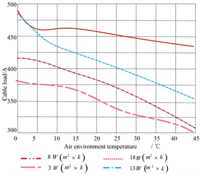
In order to analyze the change of cable ampacity with air convection heat transfer coefficient, four parameters 3W(m2×k), 8W(m2×k), 13 W(m2×k) and 18 W(m2×k) are set respectively [14].
3W(m2×k), 8W(m2×k), 13 W(m2×k) and 18 W(m2×k) are set in the software to study the relationship between the current-carrying capacity of the cable and the convection heat transfer coefficient of the air. The natural convection heat transfer coefficient of air is between 5 and 25. The ampacity of the test cable is shown in Table 1.
Table 1Current carrying capacity of cable
Heat transfer coefficient | 10 °C | 20 °C | 30 °C | 40 °C |
3W(m2×k) | 384A | 363A | 328A | 311A |
8W(m2×k) | 433A | 411A | 380A | 353A |
13W(m2×k) | 445A | 428A | 405A | 371A |
18W(m2×k) | 482A | 448A | 417A | 390A |
Temperature monitoring by using the temperature sensor cable temperature. In Table 1, if the convective heat transfer coefficient is set to a constant value, the current carrying capacity of the cable will decrease with the increase of the air temperature, and vice versa. When the air temperature is set to a constant value, the cable ampacity will increase with the increase of heat transfer coefficient, and vice versa [15]. The results are shown in Fig. 1.
Fig. 1Current carrying capacity trend
2.2. Deep layer of cable trench
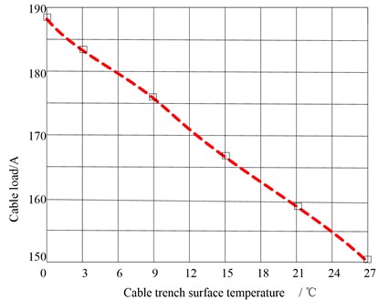
The influence of soil temperature on cable ampacity in the actual situation of the cable trench laying is that the earth temperature changes with the seasons of spring, summer, autumn and winter, which indirectly affects the cable ampacity. At this time, the soil temperature in the infinite area is particularly important. At present, the soil temperature is set at 10 ℃, 15 ℃, 20 ℃, 25 ℃ and 30 ℃ to analyze the impact on the cable ampacity [16]. The measurement results are shown in Fig. 2.
Fig. 2Relationship between ampacity and surface temperature of cable trench
2.3. Cable temperature calculation based on Whale algorithm
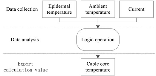
Cable laying mainly includes cable trench, direct burial, cable tray, pipe gallery laying, etc. The cable skin and ambient temperature are the essential data to calculate the temperature of the conductor core. Only the large interference variable with the temperature change is selected as the reference object, and other small interference variables are ignored [17]. As shown in Fig. 3.
Fig. 3Calculated relation of guide core temperature
2.3.1. Whale algorithm's behavior of surrounding prey
To describe the behavior of humpback whales when they surround their prey while hunting, Mirjalili proposed the following mathematical model:
where is the current number of iterations; and are the coefficients, where is the best whale position vector so far, and is the current whale position vector, where and are given by:
where and are random numbers in (0, 1). The value of a decreases linearly from 2 to 0. represents the current number of iterations, and is the maximum number of iterations.
2.3.2. Hunting behavior of whale algorithm
According to the hunting behavior of humpback whale, it swims to its prey in a spiral motion, so the mathematical model of hunting behavior is as follows:
where is the distance between the whale and the prey, is the best position vector so far, is a constant that defines the shape of the spiral, and is a random number in (−1, 1). It is worth noting that whales swim in a spiral shape to their prey while shrinking their encirclement. Therefore, in this synchronous behavior model, it is assumed that there are probability selection contraction surrounding mechanism and probability selection spiral model to update the whale's position, and its mathematical model is as follows:
When attacking the prey, the value of a is set to decrease close to the prey in the mathematical model, so that the fluctuation range of also decreases with a. When the value of a decreases from 2 to 0 in the iteration process, it is a random value within . When the value of A is within [–1, 1], the next position of the whale can be any position between its current position and the position of the prey. The algorithm assumes that when , the whale attacks the prey [18].
2.3.3. Whale algorithm to search for prey
When searching for prey, the mathematical model is as follows:
where is a randomly selected whale position vector. The algorithm sets when , randomly selects a search agent, and updates the position of other whales according to the randomly selected whale position, forcing the whale to deviate from the prey to find a better prey, which can enhance the exploration ability of the algorithm and enable the WOA (Office Automation) algorithm to carry out global search. To obtain the real cable data, it is obtained from an experiment, as shown in Fig. 4 and Table 2.
As shown in Fig. 4, among the estimated values calculated by the whale algorithm, the maximum error from the actual value is 1.05℃, and the minimum error is 0.77 ℃. The purpose of setting a set of abrupt data of 200 A current in Table 2 is to test whether the algorithm can feed back in real-time. Finally, the whale algorithm can be used after testing.
Fig. 4Relationship between the predicted value and the true value
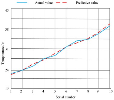
Table 2Cable test data
Number | Cable skin temperature (℃) | Cable ambient temperature (℃) | Cable current (A) | Cable conductor temperature (℃) |
1 | 24.42 | 23.14 | 115 | 24.72 |
2 | 26.43 | 25.44 | 125 | 26.62 |
3 | 28.42 | 27.63 | 135 | 28.15 |
4 | 30.42 | 29.67 | 145 | 31.35 |
5 | 32.48 | 31.49 | 155 | 33.68 |
6 | 61.30 | 59.78 | 200 | 63.72 |
7 | 37.78 | 35.39 | 165 | 38.61 |
8 | 39.92 | 37.28 | 155 | 40.05 |
9 | 42.12 | 40.08 | 145 | 43.92 |
10 | 58.17 | 56.93 | 135 | 60.72 |
3. Data testing
3.1. Data transmission stability test
The monitoring system using the ZigBee network can effectively reduce the early investment cost and later maintenance cost of the system, but the data will drop frames when transmitted through the wireless network, resulting in data loss. In addition, to determine the packet loss of the data collected by the power cable monitoring system in the transmission process, 10000 data are sent at the acquisition end. The distance between the coordinator and the router is 100 m, and the interval time is 1s [19]. Then count the number of data received by the simulated server to understand the data loss rate. The data is counted by the script written by MATLAB.
The statistical results are shown in Table 3.
Table 3Statistical table of data packet loss rate
Times | First time | Second time | Third time | Fourth time | Fifth time |
Number of data sent | 10000 | 10000 | 10000 | 10000 | 10000 |
Number of received data | 9994 | 9991 | 9995 | 9993 | 9994 |
Data loss rate | 0.06 % | 0.09 % | 0.05 % | 0.07 % | 0.06 % |
It can be seen from the statistical table of data packet loss rate in Table 3 that the average packet loss rate is only 0.066 % in the five tests. For the data transmission quantity of 10000 times, the data loss rate of 0.066 % is acceptable and will not affect the monitoring function of the system.
3.2. Data transmission optimization
The data is sent at an interval of 1 s, and there is packet loss in the data. It is necessary to avoid data loss once. The optimization process is shown in Fig. 5.
Fig. 5Data transmission optimization process
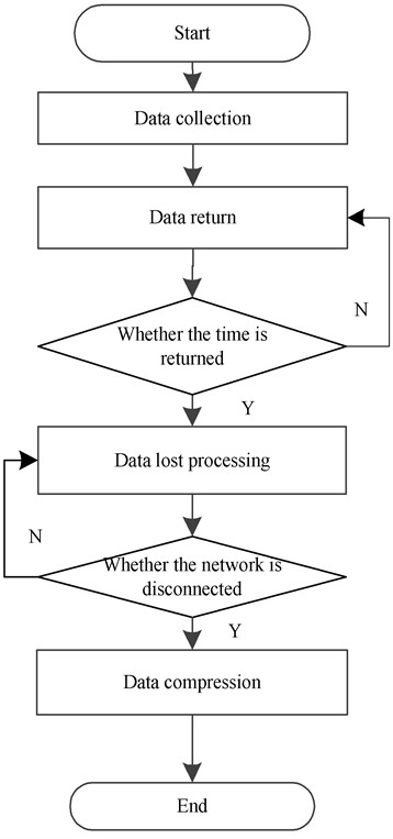
(1) Hardware code: after the data is received, it shall be returned once, and the data shall be processed only after the return is confirmed. If the return is not received within the set time, it shall be transmitted again, repeated, repeated for 4 times, then abandoned, and an error is reported. Set the time interval of uploaded data as 10 s;
(2) Software code: when the received data is incomplete, the data needs to be lost. At the same time, whether the network is disconnected is detected;
(3) Optimize the data and compress it as much as possible to reduce the amount of data sent.
4. Experimental analysis
4.1. Experimental environment
In the cable trench environment shown in Fig. 6, the upper cable is close to the wall, and the heat dissipation effect of this cable is worse than that of the lower cable.
Fig. 6Cable trench environment (From the author of the cable trench in Urumqi, Xinjiang at 10 am)
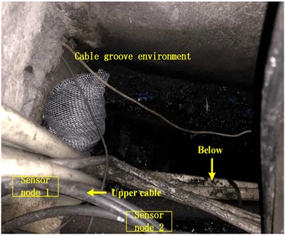
The designed sensor node is installed with this cable. Due to the experimental conditions, the selected cable trenches are very dense and the installation of nodes is difficult, so only two nodes are selected for installation [20].
The temperature and humidity of node 1 at the current moment are 19.8 ℃ and 51 %, respectively. Node 2 has a temperature of 20.6 °C and a humidity of 50 %. The temperature and humidity of the two nodes fluctuate in a very stable range. The test results are shown in Table 4 and Table 5.
Table 4Comparison of temperature results
Test results | Actual results | Error | |
Node 1 temperature (℃) | 19.8 | 18.6 | 5.7 % |
Node 2 temperature (℃) | 20.6 | 19.9 | 3.5 % |
Table 5Comparison of humidity results
Node 1 Humidity | Test results | Actual results | Error |
51 | 48 | 6.25 % | |
Node 2 Humidity | 50 | 47 | 6.38 % |
A professional temperature and humidity measuring device were used to measure the temperature and humidity on the spot, and the results were compared with the test results.
In the table of temperature and humidity tests, the two nodes have different errors. There are no two identical sensors in the manufacturing process, so the error is caused. There are also three errors in the sensor. One is the loss of the sensor circuit. The other is that the data transmission is not strictly linear, and the third is that the conversion formula integrated in the sensor also has certain errors [21].
4.2. Experimental results and analysis
The experimental steps are as follows: firstly, after the experimental platform is powered on through the switch cabinet, when the ambient temperature is 20 ℃, the currents of 100 A, 150 A, 175 A, 200 A and 245 A are loaded respectively. The temperature is measured through the temperature sensor and thermocouple. Then, the transient values of the outer surface temperature and cable core temperature under different currents are read every 25 minutes. The cable core temperature no longer changes significantly, that is, it is considered to have reached the steady-state value of cable operation. After each group of test current, the cable outer surface temperature shall be cooled to the room temperature with an error of no more than 0.5 ℃. Then, the next group of tests can be carried out. The purpose of this is to prevent the environmental temperature factors from affecting the accuracy of the test. Therefore, the steady-state temperature distribution diagram under different currents can be obtained as shown in Fig. 7.
Fig. 7Cable temperature rise test results
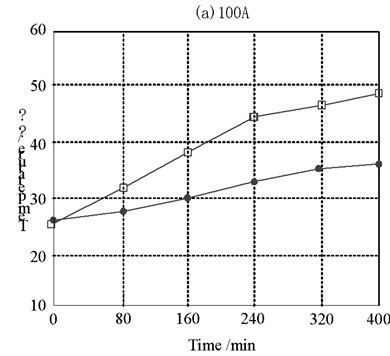
a) 175 A
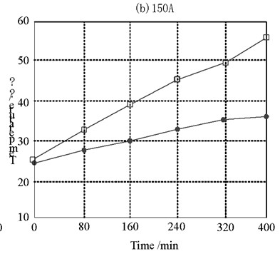
b) 200 A
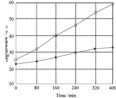
c) 175 A
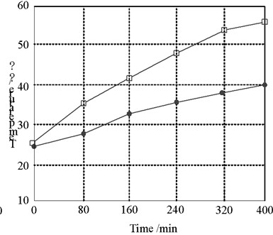
d) 200 A
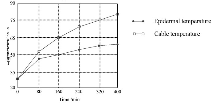
e) 245 A
It can be seen from the steady-state temperature diagram of the cable under different currents that the temperature of the cable skin and the cable core increases with the increase of the current. The larger the current carrying capacity is, the greater the temperature difference between the cable skin and the cable core is, which is consistent with the simulation conclusion of the cable temperature field.
The recorded temperature values of the cable core and outer sheath surface at the time of reaching the steady state are compared with the temperature values calculated by the finite element model, as shown in Table 6.
Table 6Comparison between experimental temperature and simulation temperature
Current value (A) | Experimental temperature (°C) | Simulate and calculate the temperature (°C) | ||
Cable core | Outer sheath | Cable core | Outer sheath | |
150 | 55.7 | 34.5 | 52.8 | 34.2 |
175 | 68.1 | 47.2 | 61.8 | 40.5 |
245 | 93.7 | 56.3 | 86.7 | 57.7 |
Table 6 shows that the temperature calculated by the finite element model is close to the temperature of the quantity, with a difference of 2.91 %. Within the value range, the whole system is in line. The temperature and humidity sensors were calibrated and the number was fixed qualitatively. The ratio of the best fruit to fruit shows that the accuracy of the system is the accuracy of the calculation.
5. Conclusions
In this paper, the temperature field is simulated according to the directly buried cable. The influence of environmental temperature on the temperature field distribution is obtained. The model of the cable body is established and the equivalent optimization is carried out. A calculation model of the monitoring parameters of the cable skin and cable core temperature based on the whale swallowing algorithm is proposed. The finite element simulation calculation formula is used for analysis. The temperature rise measurement model of the cable core conductor is obtained after optimization, and the test results are compared with the standard thermometer and hygrometer in the test process to verify the accuracy of the sensor. It is proved that the research content of this paper can be operated under different environmental temperatures. The analysis of cable temperature field distribution under different environmental temperatures has important and direct significance for the safe and effective operation of the cable.
The boundary condition considered in the simulation in this paper is the third type of boundary condition, which does not take into account that in the actual operation of the cable, there may be soil or other cables under the cable, resulting in changes in the convection heat transfer coefficient, resulting in distortion of the surrounding temperature field, which needs to be verified from a practical point of view.
References
-
P. Ocłoń et al., “Thermal performance optimization of the underground power cable system by using a modified Jaya algorithm,” International Journal of Thermal Sciences, Vol. 123, pp. 162–180, Jan. 2018, https://doi.org/10.1016/j.ijthermalsci.2017.09.015
-
L. Wang, Z. Li, J. Chen, Y. Huang, H. Zhang, and H. Qiu, “Enhanced photocatalytic degradation of methyl orange by porous graphene/ZnO nanocomposite,” Environmental Pollution, Vol. 249, pp. 801–811, Jun. 2019, https://doi.org/10.1016/j.envpol.2019.03.071
-
H. Fu et al., “Zinc oxide nanoparticle incorporated graphene oxide as sensing coating for interferometric optical microfiber for ammonia gas detection,” Sensors and Actuators B: Chemical, Vol. 254, pp. 239–247, Jan. 2018, https://doi.org/10.1016/j.snb.2017.06.067
-
Y. Zhu et al., “Fabrication of three-dimensional zinc oxide nanoflowers for high-sensitivity fiber-optic ammonia gas sensors,” Applied Optics, Vol. 57, No. 27, pp. 7924–7930, Sep. 2018, https://doi.org/10.1364/ao.57.007924
-
M. H. Jali et al., “Formaldehyde sensing using ZnO nanorods coated glass integrated with microfiber,” Optics and Laser Technology, Vol. 120, p. 105750, Dec. 2019, https://doi.org/10.1016/j.optlastec.2019.105750
-
Feng Y. et al., “ZnO-nanorod-fiber UV sensor based onevanescent field principle,” Optik, 2020, https://doi.org/10.1016/j.ijleo.2020.163672
-
S. Ebrahimi, A. Bordbar-Khiabani, and B. Yarmand, “Immobilization of rGO/ZnO hybrid composites on the Zn substrate for enhanced photocatalytic activity and corrosion stability,” Journal of Alloys and Compounds, Vol. 845, p. 156219, Dec. 2020, https://doi.org/10.1016/j.jallcom.2020.156219
-
Miao Y. P. and Yang P., “Decoration of alpha-Fe2O3 on Graphene for Photocatalytic and Super capacitive Properties,” Journal of Nanoscience and Nanotechnology, Vol. 18, No. 1, pp. 333–339, 2018.
-
Hafiz M. A. et al., “Advanced Ag/rGO/TiO2ternary nanocomposite based photoanode approaches to highly-efficientplasmonic dye-sensitized solar cells,” Optics Communications, Vol. 453, No. 15, 2019, https://doi.org/10.1016/j.jallcom.2019.124408
-
H. M. A. Javed et al., “Efficient Cu/rGO/TiO2 nanocomposite-based photoanode for highly-optimized plasmonic dye-sensitized solar cells,” Applied Nanoscience, Vol. 10, No. 7, pp. 2419–2427, Jul. 2020, https://doi.org/10.1007/s13204-020-01430-x
-
A. A. Qureshi, S. Javed, H. M. Asif Javed, A. Akram, M. Jamshaid, and A. Shaheen, “Strategic design of Cu/TiO2-based photoanode and rGO-Fe3O4-based counter electrode for optimized plasmonic dye-sensitized solar cells,” Optical Materials, Vol. 109, p. 110267, Nov. 2020, https://doi.org/10.1016/j.optmat.2020.110267
-
S. Zhou, B. Huang, and X. Shu, “A multi-core fiber based interferometer for high temperature sensing,” Measurement Science and Technology, Vol. 28, No. 4, p. 045107, Apr. 2017, https://doi.org/10.1088/1361-6501/aa5e82
-
K. Chen, Y. Yue, and Y. Tang, “Research on temperature monitoring method of cable on 10 kV railway power transmission lines based on distributed temperature sensor,” Energies, Vol. 14, No. 12, p. 3705, Jun. 2021, https://doi.org/10.3390/en14123705
-
L. Xiong, Y. Chen, Y. Jiao, J. Wang, and X. Hu, “Study on the effect of cable group laying mode on temperature field distribution and cable ampacity,” Energies, Vol. 12, No. 17, p. 3397, Sep. 2019, https://doi.org/10.3390/en12173397
-
H. Tan, F. Ling, Z. Guo, J. Li, and J. Liu, “Application of a wide-field electromagnetic method for hot dry rock exploration: a case study in the Gonghe Basin, Qinghai, China,” Minerals, Vol. 11, No. 10, p. 1105, Oct. 2021, https://doi.org/10.3390/min11101105
-
Y. Liu, S. Zhang, X. Cao, C. Zhang, and W. Li, “Simulation of electric field distribution in the XLPE insulation of a 320 kV DC cable under steady and time-varying states,” IEEE Transactions on Dielectrics and Electrical Insulation, Vol. 25, No. 3, pp. 954–964, Jun. 2018, https://doi.org/10.1109/tdei.2018.006973
-
M. Meziani, A. Mekhaldi, and M. Teguar, “Effect of space charge layers on the electric field enhancement at the physical interfaces in power cable insulation,” IEEE Transactions on Dielectrics and Electrical Insulation, Vol. 23, No. 6, pp. 3725–3733, Dec. 2016, https://doi.org/10.1109/tdei.2016.005931
-
L. Duan et al., “Heterogeneous all-solid multicore fiber based multipath Michelson interferometer for high temperature sensing,” Optics Express, Vol. 24, No. 18, p. 20210, Sep. 2016, https://doi.org/10.1364/oe.24.020210
-
Y. Zhang et al., “Conductor temperature monitoring of high-voltage cables based on electromagnetic-thermal coupling temperature analysis,” Energies, Vol. 15, No. 2, p. 525, Jan. 2022, https://doi.org/10.3390/en15020525
-
Jian Wang, Huan Jin, Zhi Yang, Bin Zhao, Xiao Ma, and Kunpeng Ji, “Study on finite element analysis of the external heat resistance of cables in duct bank,” Energy Reports, 2020.
-
J. H. Choi, C. Park, P. Cheetham, C. H. Kim, S. Pamidi, and L. Graber, “Detection of series faults in high-temperature superconducting dc power cables using machine learning,” IEEE Transactions on Applied Superconductivity, Vol. 31, No. 5, pp. 1–9, Aug. 2021, https://doi.org/10.1109/tasc.2021.3055156
About this article

The authors have not disclosed any funding.
The datasets generated during and/or analyzed during the current study are available from the corresponding author on reasonable request.
Menghao Lin: writing-original draft preparation. Qian Shi: writing-review and editing. Tianle Wang: conceptualization and methodology
The authors declare that they have no conflict of interest.
