Abstract
Aiming at the problem that five axis redundant industrial manipulator dynamic obstacle avoidance and trajectory planning algorithm does not consider the minimum difference of each joint of the manipulator, which leads to low success rate of obstacle avoidance planning, slow convergence speed of path cost and long time of obstacle avoidance planning, a simulation study on dynamic obstacle avoidance trajectory planning of five axis redundant industrial manipulator is proposed. According to the D-H rule, the coordinate system of each link joint of the five axis redundant industrial manipulator is established, and the forward and inverse kinematics of the five axis redundant industrial manipulator is analyzed. AABB's hierarchical bounding box tree algorithm is used to detect the collision of five axis redundant industrial manipulator. This paper uses harmony search algorithm to plan the obstacle avoidance path of five axis redundant industrial manipulator, determines the objective function and constraints of the optimization problem, sets algorithm parameters, initializes harmony memory, creates new harmony, updates harmony memory, checks and searches the target state, achieves the maximum number of iterations, and realizes the dynamic obstacle avoidance and trajectory planning of five axis redundant industrial manipulator. The experimental results show that the path cost of the proposed algorithm converges faster, and can effectively improve the success rate of obstacle avoidance planning and shorten the time of obstacle avoidance planning.
Highlights
- Establish joint coordinate system to realize kinematics analysis
- Layered boundary block diagram tree to avoid collision between manipulators
- Fusion and harmony search planning dynamic obstacle avoidance path
1. Introduction
At present, robot technology has become more and more mature, and its application industry has gradually expanded from mechanical manufacturing industry to aerospace, military, industrial medical and health, service industry and other industries, which plays a significant role in promoting the innovation of science and technology and production. With the development of manipulator, in order to complete more complex tasks, the number of joints has developed from single joint to multi joint, and the workspace has also been transformed from two-dimensional space to three-dimensional space [1]. Redundant manipulator has a high degree of flexibility, fault tolerance and reliability. By using its self motion characteristics, it can avoid obstacles, singular points, joint limit and optimize joint torque. Obstacle avoidance path planning is to plan a collision free path through a certain strategy in a complex working environment, so that the manipulator can successfully avoid obstacles and reach the desired position [2]. In order to ensure the manipulator to complete the task smoothly in the working environment with obstacles, the obstacle avoidance technology must be used to make the manipulator avoid obstacles without collision. Obstacle avoidance path planning has always been a concern in the field of robot control [3]. Good and effective obstacle avoidance path planning algorithm can save the working time of the manipulator, reduce the mechanical wear, and make the manipulator run safely in various working environments. Obstacle avoidance path planning and trajectory planning are of great significance for a manipulator to perform its tasks smoothly.
Obstacle avoidance motion planning is one of the research topics of robot technology. Scientific and reasonable obstacle avoidance planning is to ensure that the manipulator in the working environment can complete a specific motion with a better trajectory without collision, so as to ensure the normal operation of the manipulator. At present, there are many researches on Obstacle Avoidance Planning of manipulator. In reference [4], a general method for trajectory planning of redundant planar manipulator is proposed. The mathematical relationship between joint space and Cartesian space in two-dimensional space is derived. The joint classification method is used to obtain the corresponding joint solution. A new application of nodes in quintic B-spline curve is introduced to generate the inverse solution of type I redundant joint. The particle swarm optimization algorithm is extended to solve two kinds of redundant joints. The initial trajectories of joints and end effectors are optimized. The solution of non redundant joints is derived by using the relationship between joint space and Cartesian space. The solution of the algorithm is closer to the global optimal solution. In reference [5], a new reliable feedback motion planning algorithm is proposed to guide the spacecraft to the desired position while satisfying the dynamic and environmental constraints. The positive invariant set transformation is applied to the online sampling method based on the asymptotically optimal fast exploring random tree. Under instantaneous constraints, a series of PI sets constitute a time-varying safety corridor. When the feedback controller corresponding to PI set transformation is implemented, the spacecraft is kept in the corridor. The algorithm is effective in obstacle avoidance planning. However, the above algorithm does not consider the minimum difference of each joint of the manipulator, which leads to low success rate of obstacle avoidance planning, slow convergence speed of path cost and long time of obstacle avoidance planning.
In order to solve the above problems, a simulation study on dynamic obstacle avoidance and trajectory planning of a five axis redundant industrial robot is proposed. The technical route of the article is as follows:
Step 1: According to the D-H rule, the joint coordinate system of each link of the five axis redundant industrial manipulator is established, and the forward and inverse kinematics of the five axis redundant industrial manipulator are analyzed;
Step 2: A hierarchical bounding box tree algorithm is used to detect the collision of a five axis redundant industrial manipulator;
Step 3: The coordinated search algorithm is used to plan the obstacle avoidance path of the five axis redundant manipulator to realize the dynamic obstacle avoidance and trajectory planning of the five axis redundant robot.
Step 4: Carry out experimental analysis on the success rate of obstacle avoidance planning, the speed of path cost convergence and the time of obstacle avoidance planning;
Step 5: Conclusion.
Through the above steps, the research on the dynamic obstacle avoidance trajectory planning of the five axis redundant industrial manipulator is realized, so as to improve the success rate of obstacle avoidance planning, accelerate the speed of path cost convergence and shorten the obstacle avoidance planning time, in order to provide valuable reference and help for the development of robot technology and its application industry in the future.
2. Kinematics analysis of five-axis redundant industrial manipulator
2.1. Forward kinematics analysis of manipulator
Five axis redundant industrial manipulator mechanism consists of six joints, of which four are rotary joints and two are moving joints with the same direction. The pose of the manipulator end is determined by these six joints. According to the D-H rule [6], the coordinate system of each link joint of the robotic arm is established, and the pose of each joint is described by the four parameters , , , and . The four parameters are specifically defined as follows: is the distance from to along the axis; is the angle of rotation from to around the axis; is the distance from to along the axis; is the angle of rotation from to around the axis.
Then, the relative pose of the connecting rod in the coordinate system can be expressed as:
The parameters of five axis redundant industrial manipulator are as Table 1.
Table 1Connecting rod parameters of five axis redundant industrial manipulator
Connecting rod | / mm | / ° | / mm | / ° | Variable range |
1 | 0 | 0 | 1630 | –45~45 | |
2 | 0 | –90 | 825 | –90~–135 | |
3 | 0 | –90 | 0 | 325~2625 | |
4 | 0 | 0 | 0 | 2950~5700 | |
5 | 0 | 90 | 0 | 0~90 | |
6 | 0 | 90 | –1330 | –360~360 |
Substituting the data in Table 1 into Eq. (1), the transformation matrix between adjacent links of the robotic arm can be obtained, and the coordinate transformation matrix of the end of the robotic arm relative to the base can be obtained:
After replacing the two-angle sum formula and , the calculation result is Eq. (3):
2.2. Inverse kinematics analysis of manipulator
Inverse kinematics of the manipulator is to solve the corresponding joint variables through the pose of the end of the manipulator [7]. But the inverse kinematics equation is really a nonlinear problem, in the process of solving, it needs to couple multiple angles, especially the five axis redundant manipulator studied in this paper, there are infinitely many inverse solutions, so we need to choose a group of inverse solutions according to the actual situation. The coordinate system of each joint of five axis redundant industrial manipulator is as Fig. 1.
Fig. 1Coordinate system of each joint of five axis redundant industrial manipulator
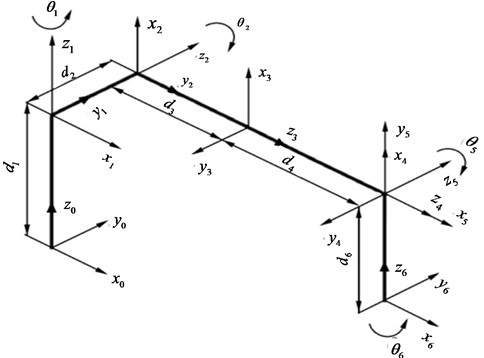
It can be seen from Fig. 1 that when changes, , , and form a plane triangle. The parameters of the triangle are also related to and . That is to say, , , , 4 parameters always have a certain functional relationship, which can be solved by closed solution method and geometric method [8]. This paper takes the closed solution method as an example to solve it.
Solving the matrix equation can be obtained:
Solving the matrix equation can be obtained:
Solving the matrix equation can be obtained:
Solving the matrix equation can be obtained:
Eqs. (4), (5), (6) and (7) are the analytical solutions of the joint variables , , , and respectively. It can be seen that can be obtained directly from the end pose of the robotic arm, but it needs to be calculated according to the range of motion and the principle of minimum motion are selected. The values of and are related to , and the value of is determined by , , and . Therefore, a set of inverse solutions can be obtained by determining the values of the four joint variables , , , and .
Taking into account the actual working conditions of the robotic arm, the joint 5 is close to the working area and the environment is harsh, and is much smaller than . The movement in the direction is mainly completed by the joints 3 and 4, and the is more complex due to the complicated calculations. The efficiency can be calculated after determining and . Therefore, the following provisions can be made:
(1) Joint 5 was kept as motionless as possible, and joint 3 and joint 4 were the main motion joints.
(2) Ensure that joint 3 and joint 4 each joint changes minimum.
In the process of solving the inverse motion, the Eq. (8) of the functional equation about is constructed according to the Eq. (5):
Determine the value of to fit the range of motion of joint 5, and then solve for and . and are calculated according to Eq. (9):
In Eq. (9), is the value of the initial posture of the robotic arm, is the value of the initial posture of the robotic arm, is the value of the initial posture of the robotic arm, 2300 and 1750 are the maximum allowable values of and respectively the amount of change. The specific solution process of , , , is as Fig. 2.
Fig. 2Reverse solution flow chart of manipulator
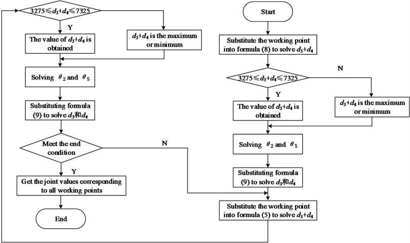
In Fig. 2, 7325 and 3275 are the maximum and minimum values of respectively. When using the above method to calculate, because the working point is selected in the working space, there is no situation where and have no solution. When solving Eq. (8), two solutions may be obtained. The range of motion of and is preferentially selected, that is, the value in the interval [3275, 7325], otherwise the minimum change value is selected according to the corresponding to the last operating point. is a monotonic function in the interval [0°, 90°], and the value of is unique. Eq. (6) is a transcendental equation. When solving, you need to replace and with . may have two values. After solving by the choice is made according to the range of motion and the principle of minimum motion.
2.3. Dynamic analysis of manipulator
The dynamic modeling of the manipulator is an essential part of the dynamic model to achieve the control purpose. The accuracy of the model has a direct impact on the trajectory planning and control accuracy of the manipulator. Newton Euler method can solve kinematics parameters and joint torque respectively through extrapolation and interpolation iteration. The whole calculation process is not only fast in calculation and easy to convert program language, but also can solve system dynamics problems with high degrees of freedom such as mechanical arm. First, the forward recursion of the manipulator is solved. The velocity and acceleration of each point are calculated in Eq. (10):
where, represents angular velocity; is the angular acceleration; represents linear acceleration; is the linear acceleration at the center of mass.The resultant force and moment at the center of mass of the connecting rod shall be calculated according to Eq. (11):
where, represents the resultant force at the center of mass of the connecting rod; represents the resultant moment at the center of mass of the connecting rod. The expression of the equation of reverse recursion is shown in Eq. (12):
where, represents the acting force at the connecting rod joint; represents the moment balance equation at the connecting rod joint; represents the joint moment of the connecting rod; represents the driving torque at the joint. in Eqs. (10), (11) and (12) represents the vector of axis in coordinate system ; represents the rotation matrix in coordinate system relative to coordinate system ; and represent the position vector of the origin of coordinate system in coordinate system and the position variable of the center of mass of the connecting rod; represents the inertia tensor of the member; , represents the force and torque acting on the actuator at the end of the mechanical arm.
3. Five-axis redundant industrial manipulator dynamic obstacle avoidance trajectory planning algorithm
3.1. Collision detection based on AABB hierarchical bounding box tree
There are all kinds of obstacles in the manipulator workspace. In order to ensure the safe operation of the manipulator and avoid unnecessary losses, collision detection is needed. In this paper, we need collision information in a given state, so we need discrete collision detection algorithm. AABB based hierarchical bounding box tree algorithm is one of the most commonly used discrete collision detection algorithms. Because of its low construction difficulty, small storage capacity, simple intersection test, and less calculation of bounding box update when the object rotates, it has been deeply studied and widely used [9]. The flow chart of AABB based hierarchical bounding box tree collision detection algorithm is as Fig. 3.
Fig. 3AABB based hierarchical bounding box tree collision detection algorithm flow
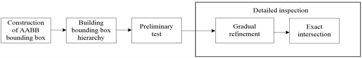
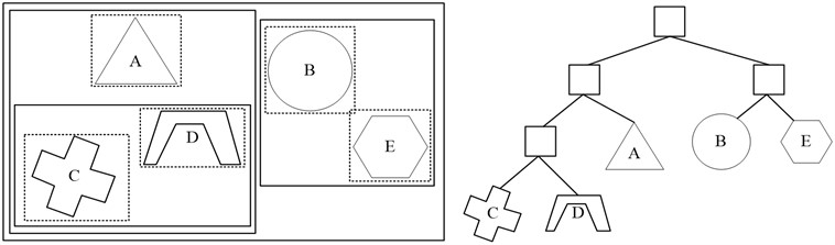
The construction of AABB bounding box is to surround an object with one or more AABB bounding boxes according to its geometric characteristics. Axis aligned bounding box (AABB) is a six sided box like cuboid in three-dimensional space (a rectangle with four sides in two-dimensional space), and its face normals are parallel to the given coordinate axis. By integrating bounding box into tree structure, namely hierarchical bounding box technology (BVH), the time of collision detection can be reduced [10]. Among them, the original bounding box set corresponds to multiple leaf nodes in the hierarchical tree, so leaf nodes can form multiple small sets, and can be limited by a larger bounding volume. This process can be executed recursively. Finally, a hierarchical tree structure will be constructed and an independent bounding box will be presented at the root node. The AABB hierarchical tree structure based on five objects is as Fig. 4.
Fig. 4AABB hierarchical tree structure based on five objects
When using hierarchical structure, if the parent node does not intersect in the collision test process, it is unnecessary to detect the child node, so as to improve the speed of collision detection. After the bounding box and its hierarchical tree structure are constructed, collision detection can be started. The first step is to exclude objects that are obviously disjoint. This process is called preliminary detection. Then, the possible intersecting objects are further detected, which is called detailed detection. In the detailed detection stage, the collision detection method between bounding boxes [11] is used to recursively detect whether there is a collision between nodes in the hierarchical tree (called the step-by-step refinement stage), until the leaf node of the tree, and further detect whether there is a collision between objects in the leaf node (the object surrounded by the bounding box) (called the accurate intersection stage).
3.2. Obstacle avoidance planning based on harmony search algorithm
Harmony search algorithm is equivalent to the music creation optimization problem, all kinds of musical instruments are equivalent to independent variables, the tone of musical instruments is equivalent to the value range of independent variables, and the evaluation index is equivalent to the objective function [12]. The basic harmony algorithm flow is as Fig. 5.
Fig. 5Flow chart of basic harmony algorithm
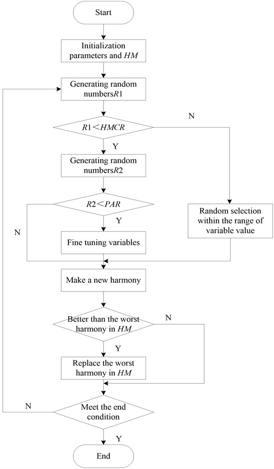
The steps of basic harmony search algorithm are as follows:
(1) The objective function and constraints of the optimization problem are determined, and the parameters of the algorithm are set.
The objective function and constraint conditions of the optimization problem are as follows:
Objective function: .
Constraints: .
(2) Initialize harmony memory:
For the solution of a function optimization problem, the harmony memory bank is usually expressed in the form of a matrix [13]. For a function to be optimized whose independent variable is dimensional, its harmony memory bank can be expressed as:
The initialization of the harmony memory bank is to randomly select the group of harmony vectors from the solution space of the objective function and calculate the respective objective function values to determine the matrix [14].
(3) Creating new harmony:
This is the most critical part of the algorithm. Creating a new harmony is to generate a new solution vector [15]. There are three ways to generate new solution vectors: learning from harmony memory, fine-tuning after learning and randomly selecting from solution space. The generation formula is as follows:
where, is a random value with a size between 0 and 1, and represents the probability of learning from the memory bank. If , the value is randomly selected from the corresponding solution space. The purpose of this is to prevent the search from falling into the local optimum or local convergence [16].
After learning and generating in the harmony search algorithm of the harmony memory bank, there is a probability of to fine-tune it. The fine-tuning formula is as follows:
where, is a random value with a size between 0 and 1, is the width of fine-tuning, and is the probability of fine-tuning.
(4) Update harmony memory.
The objective function value of the new solution vector generated in the previous step is compared with the worst objective function value in the memory. If the function value of the new solution vector is better than the worst function value, the vector corresponding to the worst function value is removed from the memory, and the new solution vector is put into the memory.
(5) Check whether the end condition is met. If not, return to step 3 to continue. Otherwise, end. The end condition can be in many forms, and the algorithm is usually terminated by setting the maximum number of iterations.
Due to the strong global convergence performance of harmony search algorithm, this paper uses harmony search algorithm to plan the obstacle avoidance path of the manipulator, and transforms the obstacle avoidance path planning problem into the problem of finding the minimum difference between the current value and the target value of each joint of the manipulator [17]. The main steps of using harmony search algorithm to search obstacle avoidance path are as follows:
Step 1: Use as the objective function and collision detection as the constraint condition to initialize the parameters of the algorithm.
Step 2: Initialize the harmony memory bank . The solution vector is randomly selected in a small neighborhood from the initial joint value of the robot arm to the target joint value , and the corresponding function value is calculated and then filled into the memory and sound library for initialization.
Step 3: Generate a new solution vector. There are three generation methods: randomly selected from the harmony memory bank , fine-tuned the solution vector selected from , and randomly selected within a small neighborhood from the current state of the robot arm to the target state .
Step 4: Update the harmony memory bank . According to the constraints, if the generated new solution vector will cause the obstacle to collide with the robotic arm, it will be discarded directly. Otherwise, the function value of the new solution vector will be compared with the worst function value in the memory bank. If the former is worse than the latter, the new solution vector is used to replace the solution vector corresponding to the latter.
Step 5: Check whether the target state is searched or the maximum number of iterations is reached. If not, continue to search. Otherwise, return to step 3 to continue. Through the above steps, the dynamic obstacle avoidance and trajectory planning of five axis redundant industrial manipulator are realized.
4. Experimental analysis
4.1. Experimental environment and data
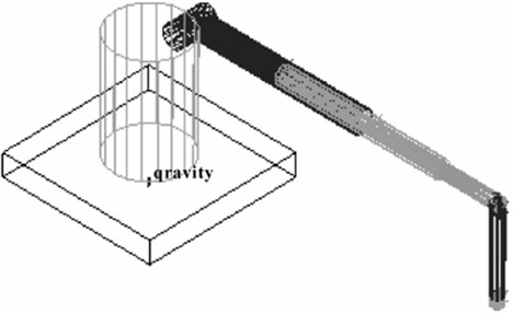
In order to verify the effectiveness of the five-axis redundant industrial manipulator dynamic obstacle avoidance and trajectory planning simulation research. Using a factory’s five-axis redundant industrial robotic arm as a prototype for simulation, the experiment was run on a computer with Intel(R) Core(TM) i3-2120 CPU @ 3.30 GHz, 4.00 GB memory, 32-bit Window 7 operating system, five-axis the simulation of the redundant industrial manipulator runs on Microsoft Visual C++ 6.0 software, and the structure model is established in the software as Fig. 6.
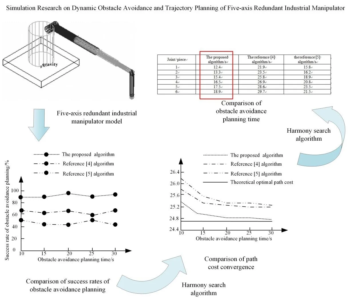
Fig. 6Five axis redundant industrial manipulator model
Due to the different paths of the dynamic obstacle avoidance and trajectory planning algorithm of the five axis redundant industrial manipulator, in order to improve the credibility of the experimental results, the experimental data in this paper is the average value of 100 times of repeated operation under the same conditions. The reference [4] algorithm, the reference [5] algorithm and the proposed algorithm are used to compare the planning success rate, the speed of convergence to the optimal value and the planning time index of different algorithms.
4.2. Comparison of success rate of obstacle avoidance planning
The success rate of obstacle avoidance planning refers to the percentage of the number of experiments to find a feasible path in 100 simulation experiments with the same planner parameters in the same planning time. In the same obstacle avoidance planning time, the comparison results of the reference [4] algorithm, the reference [5] algorithm and the proposed algorithm are as Fig. 7.
Fig. 7Comparison results of success rate of obstacle avoidance planning with different algorithms
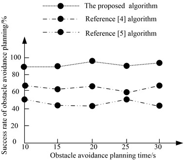
According to Fig. 7, when the obstacle avoidance planning time reaches 30 s, the average success rate of the reference [4] algorithm is 63 %, the average success rate of the reference [4] algorithm is 48 %, and the average success rate of the proposed algorithm is 92 %. Therefore, the success rate of the proposed algorithm is high.
4.3. Comparison of path cost convergence speed
On this basis, the convergence speed of the proposed algorithm is further verified. With the change of time, the path cost of the reference [4] algorithm, the reference [5] algorithm and the proposed algorithm converges to the optimal value as Fig. 8.
Fig. 8Comparison results of path cost convergence of obstacle avoidance planning with different algorithms
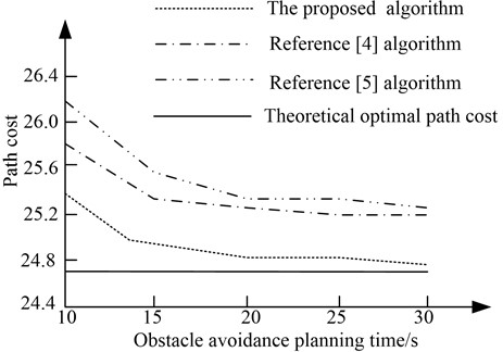
As can be seen from Fig. 8, with the increase of obstacle avoidance planning time, the path cost of different algorithms gradually converges to the theoretical optimal path generation value. However, compared with the reference [4] algorithm and the reference [5] algorithm, the path cost of the proposed algorithm is closer to the theoretical optimal path generation value, and the path cost of obstacle avoidance planning converges faster.
4.4. Comparison of obstacle avoidance planning time
In order to further verify the obstacle avoidance planning time of the five axis redundant industrial manipulator, the algorithm in reference [4], the algorithm in reference [5] and the proposed algorithm are calculated according to Eq. (13) and compared. The calculation results are shown in Table 2:
where, is the obstacle avoidance sensitivity coefficient of each joint, is the obstacle avoidance speed of each joint, is the planned route distance for obstacle avoidance of each joint, is the number of joints, .
Table 2Comparison of obstacle avoidance planning time of different algorithms
Joint / piece | The proposed algorithm / s | The reference [4] algorithm / s | the reference [5] algorithm / s |
1 | 12.4 | 21.9 | 15.8 |
2 | 13.3 | 23.5 | 16.2 |
3 | 15.4 | 25.8 | 18.9 |
4 | 16.5 | 26.9 | 20.8 |
5 | 17.5 | 28.6 | 23.5 |
6 | 18.9 | 29.7 | 21.5 |
According to the data in Table 2, when the number of joints is 6, the average obstacle avoidance planning time of the reference [4] algorithm is 29.7 s, the average obstacle avoidance planning time of the reference [5] algorithm is 20.8 s, and the average obstacle avoidance planning time of the proposed algorithm is 18.9 s. Therefore, compared with the reference [4] algorithm and the reference [5] algorithm, the obstacle avoidance planning time of the proposed algorithm is shorter.
5. Conclusions
This paper presents a simulation study on Dynamic Obstacle Avoidance Trajectory Planning of five axis redundant industrial manipulator. According to the D-H rule, the coordinate system of each link joint of the five axis redundant industrial manipulator is established, and the forward and inverse kinematics of the five axis redundant industrial manipulator is analyzed. The hierarchical bounding box tree algorithm is used to detect the collision of the five axis redundant industrial manipulator, and the harmony search algorithm is used to plan the obstacle avoidance path of the five axis redundant industrial manipulator, so as to realize the dynamic obstacle avoidance and trajectory planning of the five axis redundant industrial manipulator. The algorithm can effectively improve the success rate of obstacle avoidance planning. The average success rate can reach 92 %, and the path cost convergence speed is faster. It is closer to the convergence within 15 s, and closer to the optimal path generation value. Moreover, the algorithm class shortens the obstacle avoidance planning time, and the average maximum time is only 18.9 s. However, the algorithm does not analyze and study the bounding box with better tightness. Therefore, in the next research, we will use a more compact bounding box to build the model, and carry out the related research work for the path planning in the working environment with dynamic obstacles.
References
-
Y. Xie, X. Wu, T. Inamori, Z. Shi, X. Sun, and H. Cui, “Compensation of base disturbance using optimal trajectory planning of dual-manipulators in a space robot,” Advances in Space Research, Vol. 63, No. 3, pp. 1147–1160, Feb. 2019, https://doi.org/10.1016/j.asr.2018.10.034
-
A. Lismonde, V. Sonneville, and O. Brüls, “A geometric optimization method for the trajectory planning of flexible manipulators,” Multibody System Dynamics, Vol. 47, No. 4, pp. 347–362, Dec. 2019, https://doi.org/10.1007/s11044-019-09695-z
-
Z. Zhang, S. Chen, and S. Li, “Compatible convex-nonconvex constrained QP-based dual neural networks for motion planning of redundant robot manipulators,” IEEE Transactions on Control Systems Technology, Vol. 27, No. 3, pp. 1250–1258, May 2019, https://doi.org/10.1109/tcst.2018.2799990
-
L. Yu, K. Wang, Q. Zhang, and J. Zhang, “Trajectory planning of a redundant planar manipulator based on joint classification and particle swarm optimization algorithm,” Multibody System Dynamics, Vol. 50, No. 1, pp. 25–43, Sep. 2020, https://doi.org/10.1007/s11044-019-09720-1
-
A. Abdelaziz, R. Burton, F. Barickman, J. Martin, J. Weston, and C. E. Koksal, “Enhanced Authentication based on angle of signal arrivals,” IEEE Transactions on Vehicular Technology, Vol. 68, No. 5, pp. 4602–4614, May 2019, https://doi.org/10.1109/tvt.2019.2898898
-
Y. Ning, M. Yue, L. Yang, and X. Hou, “A trajectory planning and tracking control approach for obstacle avoidance of wheeled inverted pendulum vehicles,” International Journal of Control, Vol. 93, No. 7, pp. 1735–1744, Jul. 2020, https://doi.org/10.1080/00207179.2018.1530455
-
M. R. Benjamin, M. Defilippo, P. Robinette, and M. Novitzky, “Obstacle avoidance using multiobjective optimization and a dynamic obstacle manager,” IEEE Journal of Oceanic Engineering, Vol. 44, No. 2, pp. 331–342, Apr. 2019, https://doi.org/10.1109/joe.2019.2896504
-
J. I. Ibarreche, A. Hernández, V. Petuya, and M. Urízar, “A methodology to achieve the set of operation modes of reconfigurable parallel manipulators,” Meccanica, Vol. 54, No. 15, pp. 2507–2520, Dec. 2019, https://doi.org/10.1007/s11012-019-01081-5
-
X. Lu and Y. Jia, “Adaptive coordinated control of uncertain free-floating space manipulators with prescribed control performance,” Nonlinear Dynamics, Vol. 97, No. 2, pp. 1541–1566, Jul. 2019, https://doi.org/10.1007/s11071-019-05071-w
-
M. Galicki, “Optimal cascaded control of mobile manipulators,” Nonlinear Dynamics, Vol. 96, No. 2, pp. 1367–1389, Apr. 2019, https://doi.org/10.1007/s11071-019-04860-7
-
B. Hu, Z.-H. Guan, F. L. Lewis, and C. L. P. Chen, “Adaptive tracking control of cooperative robot manipulators with Markovian switched couplings,” IEEE Transactions on Industrial Electronics, Vol. 68, No. 3, pp. 2427–2436, Mar. 2021, https://doi.org/10.1109/tie.2020.2972451
-
T. Morales Bieze, A. Kruszewski, B. Carrez, and C. Duriez, “Design, implementation, and control of a deformable manipulator robot based on a compliant spine,” The International Journal of Robotics Research, Vol. 39, No. 14, pp. 1604–1619, Dec. 2020, https://doi.org/10.1177/0278364920910487
-
E. Franco and A. Garriga-Casanovas, “Energy-shaping control of soft continuum manipulators with in-plane disturbances,” The International Journal of Robotics Research, Vol. 40, No. 1, pp. 236–255, Jan. 2021, https://doi.org/10.1177/0278364920907679
-
Y. Ren and H. Zhao, “Improved robotic path planning based on artificial potential field method,” Computer Simulation, Vol. 37, No. 2, pp. 365–369, 2020, https://doi.org/10.3969/j.issn.1006-9348.2020.02.073
-
Y. Li and M. Zhang, “Simulation study for obstacle avoidance of autonomous underwater vehicles,” Journal of Coastal Research, Vol. 108, No. sp1, pp. 104–108, Sep. 2020, https://doi.org/10.2112/jcr-si108-021.1
-
F. Wen, N. Wu, and X. Gong, “China’s carbon emissions trading and stock returns,” Energy Economics, Vol. 86, No. 86, p. 104627, Feb. 2020, https://doi.org/10.1016/j.eneco.2019.104627
-
J. Cao, “The impact of the cross-shareholding network on extreme price movements: evidence from China,” Journal of Risk, Vol. 22, No. 2, pp. 79–102, Dec. 2019, https://doi.org/10.21314/jor.2019.423
About this article

The authors have not disclosed any funding.
The datasets generated during and/or analyzed during the current study are available from the corresponding author on reasonable request.
The authors declare that they have no conflict of interest.
