Abstract
The dynamic model of the flexible multibody systems (FMS) is usually the differential equations with time-variant, high nonlinear and strong coupling characteristics. The traditional reliability models are inefficient to solve these problems. And the reliability model is poor in accuracy and computational efficiency. Based on this point, a new stochastic surrogate model for time-variant reliability analysis of FMS is proposed. Combined model order reduction with generalized polynomial chaos, the stochastic surrogate model is established and the statistical characteristics of system responses are obtained. The calculation method of kinematic time-variant reliability is given. Finally, the effectiveness of the method is verified by a rotating flexible beam. The results show that this method has high computational accuracy compared with Monte Carlo method.
1. Introduction
The flexible multibody systems (FMS) plays an important role in many fields, such as aerospace, robotics, automobiles and so on. It has attracted much attention in recent years. In most engineering practices, the performance parameters, including material properties, geometry, stiffness, damping coefficient, manufacturing tolerances are random variables, which makes the reliability problem of FMS becomes particularly important [1]. For the time-variant reliability analysis of FMS, the traditional method is using the structural time-variant reliability theory to establish the limit state equation over a specified time period. Then Monte Carlo simulation (MCS) [2], analytical method [3], or upcrossing rate [4] can be used to analyze the time-variant reliability. However, due to the nonlinear and time-variant characteristics of the system dynamic equations, very large computational complexity causes low efficiency of using MCS method. Moreover, the limit state equation is difficult to establish under the influence of nonlinearity, which leads the analysis through analytic method and upcrossing rate method to be unsolvable [5]. Therefore, based on the surrogate model, the research of reliability analysis techniques for FMS have caused attention and achieved certain results, such as response surface method [6], neural network [7], support vector machine [8], Polynomial Chaos Expansion (PCE) [9] etc.
As an emerging the surrogate model technique, PCE belongs to stochastic mathematical models. Compared with other surrogate models, PCE, with high approximation accuracy, is not affected by the fitting point and can obtain all information of system responses. The PCE is extended by Xin and Karniadakis [10] to other classical random variables together with basis functions from the Askey-scheme. The method is called as generalized polynomial chaos (Generalized Polynomial Chaos, GPCE). GPCE is commonly used in modeling of random system, propagation and quantization of uncertainty, and solution of stochastic differential equations with arbitrary probability distribution. But for FMS with time-variant reliability analysis by GPCE are lack of research. By using PCE combined with Karhunen-Loeve expansion, Wu [11] proposes a dynamic computation method to solve FMS with material property represented by random field. Guo [12] improved nonintrusive polynomial chaos method with fuzzy probability theory is proposed for the kinematic reliability analysis of the mechanism.
Although GPCE has high accuracy, the number of random variables and the nonlinear problem caused by nonlinear and coupling characteristics, make the computational effort increased rapidly when using GPCE method for time-variant reliability analysis. Therefore, in order to improve the computational efficiency, and describe the time-variant reliability characteristic of FMS, this study propose a new time-variant reliability analysis method of FMS. The stochastic surrogate model (SSM) based on the model order reduction (MOR) method and GPCE is established to analyze uncertainty of system responses. And the method for solving the time-variant reliability is given.
2. Nonlinear model order reduction
In practice, the geometrical and physical parameters of FMS are considered as uncertain parameters. The flexible bodies are usually discrete by the finite element method (FEM). In general, the dynamic model of FMS can be established based on the hybrid coordinate method and Lagrange’s equation. The system equation of the motion with uncertain parameters can be expressed as [13]:
For the stochastic stiffness matrix , mass matrix , constraint equations and resultant force , the stochastic matrix can be represented by the truncated GPCE expansions as:
where , are generalized Askey-Wiener polynomial chaos. The total number of terms , increases rapidly with the number of stochastic parameters and the order of the polynomial chaos p [10]. The polynomials chaos are orthogonal satisfying the relationship [10]:
where denotes the inner product and is Kronecker delta. The system equation of motion can be written as:
when FEM is used to describe the deformation of the flexible bodies, the number of coordinates is very large. The dynamic model of FMS is nonlinear differential equations. In order to improve computing efficiency, the MOR method is used to reduce geometric nonlinearities of FMS, such as component mode synthesis and modern reduction schemes based on balanced truncation [14]. The common idea of the methods is to use orthogonal projection into a subspace of discretized ansatz functions [14]. Therefore, we can use an orthogonal projection onto a subspace to reduce DOFs of Eq. (4). The subspace is spanned by the columns of the orthogonal projection matrix at the mean of random variable [15]. The relationship between the reduced generalized coordinates and the original generalized coordinates is . Substituting into Eq. (4), and multiplying both sides of Eq. (4) by , the reduction of the system equation of motion can be obtained as follow:
where , , and .
3. Uncertainty analysis of system responses
3.1. The stochastic surrogate model
The GPCE method can effectively describe the uncertainty of system responses and has the function of linearization. But it also has a certain expanded order effect. For improving computing efficiency, the SSM is established by GPCE method coupled MOR method. The generalized coordinate after reduced by orthogonal projection can be represented as:
The generalized coordinate can be written in the following form as:
Let and , we have:
The size of the original GPCE problem is reduced from ∙() to ∙() and , easing the computational cost of solving the equations.
3.2. Computation of the time-variant coefficient
We use the Galerkin projection to calculate the deterministic coefficient matrix of Eq. (8). Taking inner product of both sides of Eq. (4) with respect to . The orthogonality property of is employed, we have:
Lets:
Eq. (9) can be written in Deterministic equation as:
The Eq. (10) is second-order differential equations. And the numerical integration method can be used to solve to obtain the time-variant coefficient matrix . The time-variant mean and variance of the system responses can be obtained as follows [10]:
4. Time-variant reliability analysis
In this section, the kinematic time-variant reliability of FMS will be discussed. The kinematic time-variant reliability is the probability over the life time that a system realizes its desired motion within a specific error limit. Thus, the performance function of motion error for FMS is:
where represents the desired motion output and represents the actual motion output, which can be written as . Suppose the allowable error threshold is . Thus, the time-variant limit state function is given by:
The time-variant cumulative probability of failure is given by:
In this work, the kinematic time-variant reliability of FMS is calculated by using the PHI2 method, which is the structure time-variant reliability theory. This method given in Ref.16 is realized by calculation of outcrossing rate combined with FORM method.
5. Numerical examples
5.1. Problem statement
In this section, the proposed method is validated numerically. The mechanism under consideration is a rotating flexible beam (RFM) with random variables in zero-gravity environment, as shown in Fig. 1.
The system consists of a slender Euler-Bernoulli beam and a rotating rigid hub. And the flexible beam rotates horizontally fixed to the rotating rigid hub. The drive torque is and is motion time. It is assumed that the effects of shear deformation, damping of rotor motor and gravity are negligible. In the initial state, the flexible beam is in a horizontal state without initial velocity and has no deformation. The random variables assumed to be normal distributions and be independent each other are shown in Table 3.
Fig. 1A rotating flexible beam
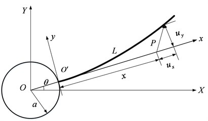
Table 1Random variables and numerical characteristics
(m) | (m) | (m) | (kg⋅m2) | (kg·m-3) | (N·m-2) | |
Mean | 0.032 | 8.5×10⁻⁴ | 0.53 | 0.0146 | 2.1×10¹¹ | 7800 |
Variance | 1×10⁻⁸ | 1×10⁻¹⁰ | 1×10⁻⁶ | 1×10-12 | 1.2×10⁸ | 100 |
5.2. Uncertainty analysis
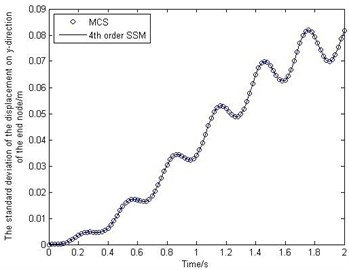
The discretization of the flexible beam into 20 elements. Each node has 2 DOFs in-plane rotation and a transverse displacement. The beam is divided into two substructures. The motion equation of RFM is established and can be written as Eq. (4) by GPCE expansions. The internal elastic DOFs are reduced by Craig-Bampton (CB) method [13]. The CB modal basis is composed of the four mode shapes and one constraint mode for each substructures. Then the modal matrix is obtained with the first five vibration modes. Consequently, the projection matrix can be calculated. Next, the stochastic surrogate model of the displacement response is established by modal basis coupled 4th order GPCE. The Newmark method simulations have been performed from 0 s to 2 s.
Fig. 2The mean and standard deviation of the deformations of the end node
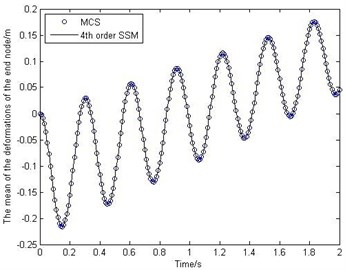
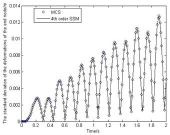
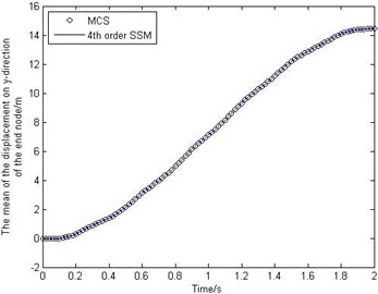
Fig. 2 shows the behavior of the mean and standard deviation of the deformations of the end node. Fig. 3 shows how the mean and standard deviation of the displacement on -direction of the end node change over time. To study the accuracy of the proposed method, MCS has been performed for 10000 times. It should be noted that from Fig. 2-Fig. 3 the stochastic surrogate model has high accuracy. And the efficiency of SSM is much higher than that of MCS, because the SSM only runs the deterministic model 1260 times, but the MCS needs to run 10000 times.
Fig. 3The mean and standard deviation of the displacement on y-direction of the end node
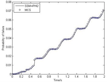
5.3. Reliability analysis
In the discussion, the response of output at the mean value of random variables is considered as the desired motion output. The time-variant limit state function is given by:
where is the actual displacement on -direction of the end node, and is the desired displacement. is assumed uniform distribution at [0, 0.85].
The kinematic time-variant reliability can be calculated with the PHI2 method. The MCS with a sample size of 10000 is also used as a benchmark for the accuracy comparison. The result is depicted in Fig. 4 and indicate that the solutions of the proposed method has certain accuracy with the relative error being less than 0.8 %.
Fig. 4The time-variant probability of failure of RFM
6. Conclusions
1) To solve time-variant reliability problem of the FMS considering nonlinear and coupling characteristics, this paper presents the stochastic surrogate model based on MOR coupled GPCE. The calculation efficiency is improved while accurate predictions on the response statistics can still be achieved. Furthermore, instead of fitting the limit state function at a particular time by using traditional reliability models, such as response surface method, the SSM in this paper is to describe directly the time-variant stochastic response characteristics of FMS over a specified time period.
2) On the basis of the SSM, the linearized time-variant limit state function of the SSM can be established directly. Then the outcrossing rate method for calculating the time-variant cumulative failure probability of failure is given.
3) Taking a rotating flexible beam for example, the feasibility and validity of the proposed method are verified. It is indicated that the calculation accuracy of the proposed method is almost the same as the MCS.
References
-
Sandu A., Sandu C., Ahmadian M. Modeling multibody systems with uncertainties. Part I: Theoretical and computational aspects. Multibody System Dynamics, Vol. 15, Issue 4, 2006, p. 369-391.
-
Xu W., Zhang Q. Probabilistic analysis and Monte Carlo simulation of the kinematic error in a spatial linkage. Mechanism and Machine Theory, Vol. 24, Issue 1, 1989, p. 19-27.
-
Wang J., Zhang J., Du X.P. Hybrid dimension reduction for mechanism reliability analysis with random joint clearances. Mechanism and Machine Theory, Vol. 46, Issue 10, 2011, p. 1396-1410.
-
Hu Z., Du X. P. Time-dependent reliability analysis with joint upcrossing rates. Structural and Multidisciplinary Optimization, Vol. 48, Issue 5, 2013, p. 893-907.
-
Hu Z., Du X. P. First order reliability method for time-variant problems using series expansions. Structural and Multidisciplinary Optimization, Vol. 51, Issue 1, 2015, p. 1-21.
-
Zhang C. Y., Bai G. C. Extremum response surface method of reliability analysis on two-link flexible robot manipulator. Journal of Central South University, Vol. 18, Issue 1, 2012, p. 101-107.
-
Xiao J., He L., Huang H. Z., Zhang X., Wang Z. Reliability analysis of elastic link mechanism based on BP neural network. International Conference on Quality, Reliability, Risk, Maintenance, and Safety Engineering, Chengdu, China, 2012, p. 286-289.
-
Ke X. W., Hou J., Chen T. F. Reliability analysis for link mechanism under influence of multiple factors based on support vector machine. Advanced Materials Research, Vol. 753, Issue 755, 2013, p. 2904-2907.
-
Shi W. S., Guo J. B., Zeng S. K., Ma J. M. A mechanism reliability analysis method based on polynomial chaos expansion. 9th International Conference on Reliability, Maintainability and Safety, Guiyang, China, 2011, p. 110-115.
-
Xiu D. B., Karniadakis G. E. The Wiener-Askey polynomial chaos for stochastic differential equations. Society for Industrial and Applied Mathematics, Vol. 24, Issue 2, 2002, p. 619-644.
-
Wu J. L., Luo Z., Zhang N., Zhang Y. Q. Dynamic computation of flexible multibody system with uncertain material properties. Nonlinear Dynamics, Vol. 85, Issue 2, 2016, p. 1231-1254.
-
Guo J. B., Wang Y., Zeng S. K. Nonintrusive-polynomial-chaos-based kinematic reliability analysis for mechanisms with mixed uncertainty. Advances in Mechanical Engineering, Vol. 10, 2014, p. 1-12.
-
Wu L., Tiso P. Nonlinear model order reduction for flexible multibody dynamics: a modal derivatives approach. Multibody System Dynamics, Vol. 36, Issue 4, 2016, p. 405-425.
-
Holzwarth P., Eberhard P. SVD-based improvements for component mode synthesis in elastic multibody systems. European Journal of Mechanics A/Solids, Vol. 49, 2015, p. 408-418.
-
Sarsri D., Azrar L., Jebbouri A., Hami A. E. Component mode synthesis and polynomial chaos expansions for stochastic frequency functions of large linear FE models. Computers and Structures, Vol. 89, Issue 3, 2011, p. 346-356.
-
Mejri M., Cazuguel M., Cognard J. Y. A time-variant reliability approach for ageing marine structures with non-linear behavior. Computers and Structures, Vol. 89, Issues 19-20, 2011, p. 1743-1753.
About this article

