Abstract
Direct transcription has been employed to transcribe the optimal control problem into a nonlinear programming problem. This paper presents a trajectory optimization method based on a combination of the direct transcription and mesh refinement algorithm. Hermite-Simpson method has the advantage of reasonable accuracy with highly sparse Hessian matrix and constraint Jacobians, and the pseudospectral method provides spectral accuracy for optimal control problems. The optimal control problem is discretized at a series of Legendre-Gauss-Lobatto points, then the trajectory states are approximated by using local Hermite interpolating polynomials. Thus, the method produces significantly smaller mesh size with a higher accuracy tolerance solution. The derived relative error estimation is then used to trade the number of mesh polynomials degree within each mesh interval with the number of mesh intervals. As a result, the suggested method can produce more small mesh size, requires less computation solution for the same optimal control problem. The simulation experiment results show that the suggested method has many advantages.
1. Introduction
Direct methods have been widely applied for the numerical solution of nonlinear optimal control problems [1-3]. The state and control of the optimal control problems are discretized at a series of suitable points in a direct method, then the continuous-time optimal control is converted into a finite dimensional nonlinear programming problem (NLP), the resulting NLP can be solved by NLP solver software [4].
With the raid development of computer technology, direct method is more and more widely applied to trajectory optimization problems [5-6], however, the low computational performance and accuracy make it difficult to use for real-time calculations. Therefore, the pseudospectral (PS) method has the advantage of high rate of convergence and large convergence radius [7-8], and provides spectral accuracy for smooth problems, but produces much denser constraints Jacobian as compared with other methods. In order to increase the sparsity of constraints Jacobians in PS method, Ross and Fahroo introduce the concepts of the knots for the Legendre PS method [9], Poustini et al. develop a trajectory optimization method based on some combination of the direct optimization method and differential flatness theory [10]. Some researchers combine the PS method and heuristic optimization method to improve trajectory method [11, 12], other researchers improve the adaptive mesh refinement algorithm to obtain higher accuracy solution with less computation time [6, 13-16]. Lei et al. develop an adaptive mesh refinement of hp PS method, the high accuracy and efficiency can be achieved by adaptive mesh refinement strategy [14]. Among the above methods, the Hermite-Simpson method has the advantage of reasonable accuracy with highly sparse Hessian matrix and constraint Jacobians [15-16]. Herman and Conway propose an additional high-order methods, however, when the Hermite interpolating polynomials extended to arbitrary higher orders [3], the framework needs more detailed derivation.
The purpose of this paper is to provide an alternative method to produce an optimal trajectory as based on a combination of the direct transcription and mesh refinement algorithm. The optimal control problem is discretized at a series of Legendre-Gauss-Lobatto (LGL) collocation points, then the state trajectories are approximated by using local Hermite interpolating polynomials, that the method in this paper is referred to as the Hermite-Legendre-Gauss-Lobatto (HLGL) method. It is noted that Williams provides a framework for arbitrary order and arbitrary number of intervals for implementation on digital computers [16]. It can be known from Ref. [16] that better accuracy can be achieved by increasing mesh polynomial degree for smooth regions, and increasing the number of subintervals for the corresponding nonsmooth regions of the solution. However, it is a fact that smooth regions and nonsmooth regions together exist in one solution of the problem. As the mesh polynomial degree and the number of mesh intervals are preset and the mesh polynomial degree are the same within each subinterval in Ref. [16], it is difficult to determine the mesh polynomial degree and the number of mesh intervals for that situation. Motived by the desire to trade the number of mesh polynomial degree with the number of mesh intervals, we develop an adaptive mesh refinement method based on direct transcription. A key contribution of this paper is that both mesh polynomial degree and the number of mesh intervals are allowed to vary, and the mesh polynomial degree within each mesh interval is not necessarily equal. Furthermore, the method also can improve computational efficiency by reducing the size of the mesh.
2. Optimal control problem
Without loss of generality, consider the following optimal control problems with inequality path constraints:
Subject to the constraints:
here the term denotes the state, and the term denotes the control. In the Eqs. (1-4), the time domain is transformed from the time domain by the following affine transformation:
where the terms and are represent for initial time and terminal time respectively. The basic idea of the approach is based on interpolating functions for state and costate on LGL quadrature nodes [17]. As the LGL nodes points are distributed over the interval [–1, 1], so it will be useful to transform the time interval.
The optimal control problem is described as to find the control variables that making sure the performance index Eq. (5) is minimized, subject to the state Eq. (2), path constraints Eq. (3) and boundary conditions Eq. (4).
3. Adaptive mesh refinement methodology
3.1. Numerical discretization and approximation
The domain is divided into mesh subintervals when using mesh refinement method. Then we have:
The mesh points have the property. The state in the subintervals is approximated by the Hermite interpolating polynomial with nth order [9]:
For ensure the integration accuracy and interpolation accuracy, the collocation points and nodes are defined as LGL points within each interval. Note that there is no distinction between collocation points and nodes in some PS method [2], whereas the collocation points are used to formulate the residual equations for the NLP, and the nodes are used to form the interpolating polynomial in this paper. Thus, the collocations points and nodes defined according to:
Note that the values of the states and states derivatives at the points determine the Hermite interpolating coefficients :
where the interval length is defined by .
It is noted that the left side of Eq. (9) determined by the number and location of the nodes. Let , then , where is the matrix on the right side of Eq. (9), and is the vector of the left side of Eq. (9). Then we have:
Differentiating in Eq. (10) with respect to , we obtain:
where:
The system constraints in per interval can be expressed as:
where:
The cost function is approximated by Gauss-Lobatto quadrature rule as:
where the term is the same as the in Ref. [16].
3.2. Approximation of solution error
The estimate method for the relative error is similar to the error estimate obtained for numerically solving a differential equation through using the modified Euler Runge-Kutta scheme. Suppose the NLP of Eqs. (1-4) on a mesh , with HLGL points has been solved. The ensuing mesh with HLGL points .
where:
Assume further that are the values of the state approximation at . We then have:
The absolute error and the relative error approximations at of the state are defined, respectively, as:
The maximum relative error in is then defined as:
3.3. Refining the mesh
If a mesh interval has met the accuracy tolerance, that is , where is the desired relative tolerance, then mesh size is reduced by decreasing mesh polynomial degree or merging adjacent mesh interval, otherwise the mesh size need to be modified by increasing points or dividing the mesh interval into several subintervals. Let be the curvature of the th component of the state in mesh interval , as:
Let and be the mean and maximum value of , respectively. Then define as the ratio of the maximum to the mean curvature:
When , and if , where is a user-defined parameter, the curvature is considered uniform in this interval mesh then the number of collocation points should be increased in interval . Let and denote the number of collocation points in interval at mesh and respectively, where is the mesh refinement iteration number. The number of points at mesh is calculated by the equation:
It is noted in Eq. (21) that the ratio of the maximum to the error tolerance have a direct effect on polynomial degree in mesh interval. An upper limit is set for the maximum allowable polynomial degree to make sure that the number of collocation points does not grow an unreasonably large value. If (i.e.exceeds the maximum allowable polynomial degree), then the mesh interval must be divided into equally spaced subintervals.
3.4. Generation of new mesh segment
Assume and , then the th mesh interval should be refined. The following procedure is the strategy for mesh interval division. Firstly, the predicted polynomial determines the number of all the collocation points in the new subinterval. Secondly, the number of collocation points should be no fewer than the minimum allowable number. In other words, whenever dividing a mesh interval, each interval will contain at least collocation points. Third, the new number of mesh intervals , is given by the equation:
where is a user-defined positive integer. In this process, it is ensured that the number of new intervals should be at least two. Thus, the number of new subintervals, denoted as , can be rewritten as:
3.5. Reducing the number of collocation points in a mesh interval
The relative error of the mesh interval is less than the desired relative tolerance, and if , then the number of collocation points should be decreased. The number of points at mesh is calculated by the equation:
3.6. Merging adjacent mesh subintervals
Before the adjacent mesh subintervals merging, it is necessary to decrease the number of each interval according to the method in Section 3.5, then generally estimate the number of mesh interval points. If , the mesh intervals and cannot be merged because highest polynomial order of the two adjacent mesh intervals are not equal. All the matching points of the original two mesh intervals are combined, and the conditions for the merging of the two mesh subintervals are mainly three:
(1) The two mesh subintervals must be adjacent.
(2) The relative error estimations of the two grid intervals are not more than .
(3) The relative error of the new mesh interval after the merger is not larger than .
3.7. Mesh refinement method
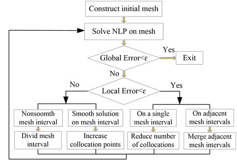
The schematic of adaptive mesh refinement method is shown in Fig. 1. The adaptive mesh refinement method is summarized as follows.
Step 1: Set 0 and supply initial mesh, , where .
Step 2: Solve NLP on current mesh .
Step 3: Compute maximum relative error in , , if for all or , then quit. Otherwise, proceed to Step 4.
Step 4: If , , proceed to Step 5, otherwise, proceed to Step 6.
Step 5: Compute the ratio between the maximum and the mean curvature in , if , set the number of collocation points increase by , else divide the interval into subintervals, where is given by Eq. (23). Then proceed to Step 7.
Step 6: For the single mesh interval, decrease the number of collocation points. Merge the adjacent mesh interval if they satisfy the conditions of the merger.
Step 7: Set , and return to Step 2.
4. Numerical example
The order and intervals of the method in Ref. [16] are fixed in each simulation, while that of the method described in this paper are variable. For the convenience of narration, the mesh refinement method in Ref. [16] is called FOI (fixed order and intervals) method, and the method in section is called VOI (variable order and intervals) method. The term denotes the mesh refinement iteration, and 0 means the mesh initialization, and the term and term denote the total collocation points and interval number respectively. The number of collocation points within each intervals of the two method is at least 2. The maximum of all mesh interval allowable error values is , where 10-6. When the mesh is initialization, the whole mesh is divided into 10 intervals, and each interval with a number of 2 collocation points. The value of term is 1.2, and the maximum number of collocation points with each interval is 12. The simulation of this paper was performed on a 3.4 GHz Intel Core i7 CPU computer and MATLAB Version R2013.
Fig. 1Schematic of adaptive mesh refinement method
4.1. Example 1
Consider the following Bang-Bang optimal control problem from Ref. [18] to illustrate the effectiveness of the method in this paper. Firstly, the method is able to accurately solve the optimal control problem. Secondly, the mesh refinement with elimination of unnecessary mesh points is able to improve the algorithm performance.
Minimize the cost function:
The analytic solution for this optimal control problem is given as:
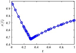
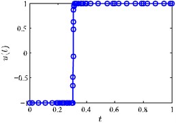
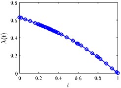
Fig. 2(a) and Fig. 2(b) and Fig. 2(c) show the exact solutions of the optimal control problem.
Fig. 2a) x(t) vs. t, b) u(t) vs. t, c) λ(t) vs. t
a)
b)
c)
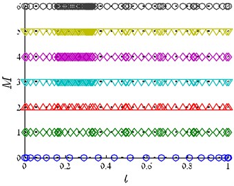
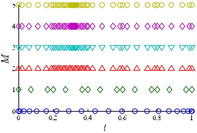
Fig. 3(a) and Fig. 3(b) show the collocation point’s distribution of the solutions obtained using FOI method and VOI method respectively. According to the exact solutions of Eq. (29), we can know that near time , the state variables and control variables are rather changeable. Fig. 4(a) and Fig. 4(b) show the collocation points are mainly located near instead of located at both ends of the solution, which is because more number of collocation points are needed to capture the changes at of the solution. When , the mesh point in Fig. 3(b) does not increase with each mesh iteration, but decreases. This is because the VOI method has the properties of reducing the interval number and the number of mesh points, and the FOI method does not have this kind of property, and mesh points in Fig. 3(a) is fixed. The iteration program is terminated at 5 when the accuracy tolerance is satisfied, and the number of mesh points using the VOI method is 60.
Fig. 3a) FOI mesh point history, b) VOI mesh point history
a)
b)
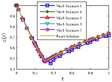
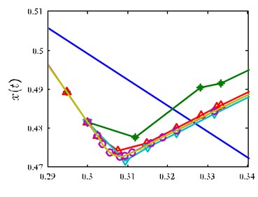
Next, we analyze the approximation ability of solution obtained by the VOI method to the exact solution. Fig. 4(a) and Fig. 4(b) show the state on each mesh refinement iteration alongside the analytic solution using the VOI method. In addition, it is seen from Fig. 4(a) show that the resulting solution gradually converge to the exact solution with each mesh refinement iteration. Fig. 4(b) shows the states near on each mesh refinement iteration, it is apparent that the difference between Mesh Iteration 1 and Analytic Solution is great, and the Mesh Iteration 2 is much closer to the analytic than Mesh Iteration 1, moreover, the gap between Mesh Iteration 2 and Mesh Iteration 3-5 is very small, which mean that the solutions are gradually converged on the analytic solution with each mesh refinement iteration. The number of mesh points near is also increasing with the continuous refinement of the mesh, because there are larger state changes near , thus the precise requirement of the solution is satisfied with more mesh points.
Fig. 4a) x(t) vs. t, b) x(t) vs. t
a)
b)
A comparison of the implementation of the VOI method and FOI method with different higher-order and intervals solutions are given in Table 1. Comparisons are made in terms of computation time, the number of total mesh points and the number of mesh intervals and the number of mesh refinement iteration , and the cost function values. In each case, the initial guesses are randomized controls, with randomized state. A total of 100 samples are used to produce the results in this paper. The terminology VOI (2, 12) refers to the VOI method where the number of mesh points within each interval can vary between 2 and 12, furthermore, the number of mesh intervals in VOI method can vary as well. All the simulations parameters are shown in Table 1, and all the results are shown in blue. As it can be seen from the results listed in Table 1, the VOI method result in the smallest overall times compared with other cases. The reason is that the VOI method has the properties of reducing the unnecessary points and intervals, while FOI method (other cases) doesn’t have this kind of property but only keeps the number of mesh points and intervals fixed until the simulation terminated. It is a fact computation times are mostly depended on the number of mesh refinement iterations and mesh size, while the growth of computation time for case 4, 7, 10 are due mostly to the increase in number of mesh points and mesh intervals. Interestingly, the number of mesh intervals in case 1 is not set parameter but the result from the simulation, where the number of mesh intervals in case 2-10 are set parameters. The case 10 using 9 mesh points with 15 intervals gives a terminal cost function of 0.4572, which is the most optimality one in all cases. The results show, as expected, that using larger mesh size results in improvements in accuracy at the expense of increases in runtime, due to the denser Jacobians. For FOI method, better accuracy can be achieved by increasing mesh points for smooth problems, whereas increasing the number of intervals to achieve better accuracy for nonsmooth problems [16]. However, it is a fact that smooth regions and nonsmooth regions together exist in one solution of the problem, so it is difficult to trade the number of mesh points and the number of mesh intervals when solving a complicated problem. The simulations show that the VOI method can trade the number of mesh points within intervals with the number of mesh intervals, and obtain an accurate solution with a relatively small mesh size.
Table 1Mesh refinement results for example1 using VOI and FOI methods
Case | Mean times / s | Cost function | Constraint Jacobian density (%) | |||||
1 | VOI | (2,12) | 13 | 1.76 | 60 | 4 | 0.4574 | 1.358 |
2 | FOI | 5 | 10 | 8.39 | 50 | 7 | 0.4589 | 3.683 |
3 | FOI | 5 | 15 | 11.3 | 75 | 6 | 0.4583 | 2.776 |
4 | FOI | 5 | 20 | 29.5 | 100 | 6 | 0.4577 | 2.103 |
5 | FOI | 7 | 8 | 10.3 | 56 | 7 | 0.4581 | 4.156 |
6 | FOI | 7 | 12 | 23.2 | 84 | 6 | 0.4575 | 3.917 |
7 | FOI | 7 | 16 | 37.2 | 112 | 5 | 0.4583 | 2.843 |
8 | FOI | 9 | 6 | 11.5 | 54 | 7 | 0.4582 | 4.468 |
9 | FOI | 9 | 10 | 25.4 | 90 | 6 | 0.4577 | 4.015 |
10 | FOI | 9 | 15 | 45.8 | 135 | 5 | 0.4572 | 3.672 |
Table 2Convergence of VOI method compare with FOI method in Ref. [16]
VOI (case 1) | FOI (case 2) | FOI (case 7) | FOI (case 10) | |||||
1 | 2.08×100 | 5.07×10⁻³ | 5.61×10⁻¹ | 4.28×10⁻³ | 1.33×100 | 3.11×10⁻³ | 1.89×10⁻¹ | 5.40×10⁻³ |
2 | 5.44×10⁻¹ | 3.22×10⁻² | 3.24×10⁻¹ | 3.19×10⁻² | 2.03×10⁻¹ | 2.58×10⁻² | 9.19×10⁻² | 7.13×10⁻² |
3 | 3.15×10⁻³ | 4.81×10⁻² | 7.53×10⁻² | 4.51×10⁻² | 4.59×10⁻³ | 4.50×10⁻² | 5.71×10⁻³ | 6.24×10⁻³ |
4 | 1.36×10⁻⁸ | 1.02×10⁻⁷ | 6.45×10⁻³ | 6.77×10⁻³ | 4.78×10⁻⁵ | 6.26×10⁻⁴ | 4.55×10⁻⁵ | 4.12×10⁻⁵ |
5 | – | – | 3.05×10⁻³ | 8.05×10⁻³ | 6.84×10⁻⁸ | 1.13×10⁻⁷ | 6.50×10⁻⁹ | 9.87×10⁻⁹ |
6 | – | – | 4.85×10⁻⁵ | 5.83×10⁻⁵ | – | – | – | – |
7 | – | – | 9.34×10⁻⁸ | 1.29×10⁻⁷ | – | – | – | – |
Next, we analyze the convergence of mesh refinement. Table 2 shows the estimated maximum relative errors and exact relative errors for each mesh refinement iteration by using the VOI method (case 1) and FOI method (case 2, 7, 10). First, it can be seen from the Table 2 that the relative error on final mesh is quite small at 10-7 for the state. The consistency in the exact relative error and the relative error approximation demonstrates the accuracy of the estimate derived in section 3.2.
4.2. Example 2
Consider the following trajectory optimization problem taken from Ref. [19] of maximizing the downrange of a Maneuverable Research Re-entry Vehicle (MaRRV). Minimize the cost function:
The state equations for hypersonic vehicle which is commonly used in midcourse guidance systems are listed as followings:
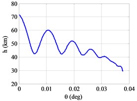
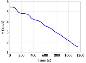
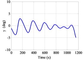
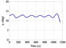
It is noted that the model (physical model and wing-body vehicle model) are taken from Ref. [19]. The initial conditions and terminal constraints are listed in Table 3. A typical solution of this problem is shown in Fig. 5(a)-(d) by using the VOI (2, 12) method.
It is seen that the solution to this example is relative smooth, especially the control variable (attack angle) is slowly changing in Fig. 5(d), meaning that it is easier to apply to engineering. As a result, it is possible to achieve an accurate solution with a relatively small number of mesh points when compared with FOI method. Table 3 shows that the terminal constraints are satisfied with error of less than 0.5 % in all parameters. A comparison of the implementation of the VOI method and FOI method solutions are given in Table 4.
Fig. 5a) Altitude vs. downrange, b) velocity vs. time, c) flight path angle vs. time, d) attack angle vs. time
a)
b)
c)
d)
Table 3Conditions and results
State variables | (km) | (deg) | (deg) | (km/s) | (deg) | (deg) |
Initial conditions | 72 | 0 | 0 | 5.435 | –1 | 0 |
Terminal constraints | 29.390 | Index | 0 | 1.500 | –5 | 0 |
Final conditions | 29.385 | 37.728 | 0.001 | 1.548 | –5.001 | 0 |
Difference | 0.005 | – | 0.001 | 0.002 | 0.001 | 0 |
It is seen that the VOI (2, 11) and FOI (5, 55) methods [shown in Table 4] are almost the most computationally efficient. FOI (9, 45) method takes the most time (with 185.7 seconds), while FOI (7, 55) produce the most optimal solution with the smallest cost function. As a result, for the vast majority of the solution, the largest decrease in error is achieved by using more mesh intervals and more mesh points in each mesh interval. The reason for more computation time needed to obtain the desired solution is that the number of mesh intervals and mesh points in each mesh interval are fixed when uses FOI methods. The simulations show that the proposed method can efficiently obtain a reliable, accurate solution for re-entry trajectory optimization problem of MaRRV.
Table 4Mesh refinement results for example2 using VOI and FOI methods
Case | Methods | Mean times / s | Cost function | ||||
1 | VOI | (2, 11) | 69 | 18.6 | 233 | 5 | –37.728 |
2 | FOI | 5 | 55 | 21.5 | 265 | 7 | –37.713 |
3 | FOI | 5 | 70 | 41.3 | 350 | 6 | –37.722 |
4 | FOI | 7 | 50 | 65.1 | 350 | 7 | –37.698 |
5 | FOI | 7 | 55 | 147.8 | 385 | 8 | –37.740 |
6 | FOI | 9 | 40 | 108.0 | 360 | 8 | –37.681 |
7 | FOI | 9 | 45 | 185.7 | 405 | 7 | –37.730 |
5. Conclusions
Trajectory optimization was considered through the combination of the direct transcription and mesh refinement approach in this paper. The suggested method uses the Hermite interpolating polynomials to approximate the trajectory states, which employ the HGL points as collocation and interpolation points. The Hermite interpolating polynomials method can improve the sparsity of the constraint Jacobian. The method employs mesh refinement algorithms that it gets the ability to trade mesh polynomial degree with the number of mesh intervals. The number of mesh interval is increased in nonsmooth regions of the solution, while the mesh points increased in smooth regions of the solution. Furthermore, the mesh size can be decreased either by reducing the mesh points or by combining adjacent mesh intervals which share the same number of mesh points. The method is applied successfully to hyper-sensitive optimal control problem and trajectory optimization problem from the open literature. It is obvious that in terms of the example reviewed, better performance is achieved when compared with other mesh refinement methods. It may be suggested to study the advantages vs. disadvantages for the method in detail in the near future compared with other conventional methods in case of mesh refinement algorithms as well about other related aspects.
References
-
Betts J. T. Survey of numerical methods for trajectory optimization. Journal of Guidance, Control, and Dynamics, Vol. 21, Issue 2, 1998, p. 193-207.
-
Elnagar G., Kazemi M. A., Razzaghi M. The pseudospectral legendre method for discretizing optimal control problems. IEEE Transactions on Automatic Control, Vol. 40, Issue 10, 1995, p. 1793-1796.
-
Herman A. L., Conway B. A. Direct optimization using collocation based on high-order Gauss-Lobatto quadrature rules. Journal of Guidance, Control, and Dynamics, Vol. 19, Issue 3, 1996, p. 592-599.
-
Gill P. E., Wong E., Murray W., Saunders M. A. User’s guide for SNOPT version 7.4: software for large-scale nonlinear programming. Numerical Analysis Report, Department of Mathematics, University of California, San Diego, 2015.
-
Soler M., Olivares A., Staffetti E. Multiphase optimal control framework for commercial aircraft four-dimensional flight-planning problems. Journal of Aircraft, Vol. 52, Issue 1, 2015, p. 274-286.
-
Arribas D. G., Rivo M. S., Arnedo M. S. Optimization of path-constrained systems using pseudospectral methods applied to aircraft trajectory planning. IFAC-PapersOnLine, Vol. 48, Issue 9, 2015, p. 192-197.
-
Huntington G. T. Advancement and analysis of a Gauss pseudospectral transcription for optimal control problems. Massachusetts Institute of Technology, Cambridge, 2007.
-
Huntington G. T., Benson D., Rao A. V. A comparison of accuracy and computational efficiency of three pseudospectral methods. AIAA Guidance, Navigation and Control Conference and Exhibit, South Carolina, 2007.
-
Ross I. M., Fahroo F. Pseudospectral knotting methods for solving nonsmooth optimal control problems. Journal of Guidance, Control, and Dynamics, Vol. 27, Issue 3, 2004, p. 397-405.
-
Poustini M. J., Esmaelzadeh R., Adami A. A new approach to trajectory optimization based on direct transcription and differential flatness. Acta Astronautica, Vol. 107, 2015, p. 1-13.
-
Su Zikang, Wang Honglun A novel robust hybrid gravitational search algorithm for reusable launch vehicle approach and landing trajectory optimization. Neurocomputing, Vol. 162, 2015, p. 116-127.
-
Ma Lin, Chen Weifeng, Song Zhengyu, Shao Zhijiang A unified trajectory optimization framework for lunar ascent. Advances in Engineering Software, Vol. 94, 2016, p. 32-45.
-
Chai Dong, Fang Yang-Wang, Wu You-li, Xu Su-hui Boost-skipping trajectory optimization for air-breathing hypersonic missile. Aerospace Science and Technology, Vol. 46, 2015, p. 506-513.
-
Lei H. M., Liu T., Li J., Jiang Z. P. Adaptive mesh refinement of hp pseudospectral method using size reduction. Control Theory and Applications, Vol. 33, 8, p. 1061-1067.
-
Ross I. M., Fahroo F. Legendre Pseudospectral Approximations of Optimal Control Problems. Lecture Notes in Control and Information Sciences, Springer-Verlag, Berlin, Vol. 295, 2003, p. 327-342.
-
Paul W. Hermite-Legendre-Gauss-Lobatto direct transcription in trajectory optimization. Journal of Guidance, Control, and Dynamics, Vol. 32, Issue 4, 2009, p. 1392-1395.
-
Garg D., Patterson M. A., Darby C. L., Francolin C., Huntington G. T., Hager W. W., Rao A. V. Direct trajectory optimization and costate Estimation of finite-horizon and infinite-horizon optimal control problems via a Radau pseudospectral method. Computational Optimization and Applications, Vol. 49, Issue 2, 2011, p. 335-358.
-
Hu Y. Q., Liu X. G., Xue A. K. A penalty method for solving inequality path constrained optimal control problems. Acta Automatica Sinca, Vol. 39, 12, p. 1996-2001.
-
Rizvi S. Tauqeer ul Islam, He Linshu, Naseemullah Vehicle performance tradeoff study for a small size lifting reentry vehicle. Proceedings of 10th International Bhurban Conference on Applied Sciences and Technology, Islamabad, Pakistan, 2013.
About this article

Supported by National Natural Science Foundation of China (61573374, 61503408).
