Abstract
This work is a comparison of the calculated and experimental natural frequencies of coil springs under the action of axial tension-compression. To calculate the coil springs, the finite element form of a single coil is proposed. The initial stiffness matrix and initial mass matrix are calculated by the differential equations of Kirchhoff-Clebsch. The co-rotational approach of single coil finite element is provided to make it applicable for calculating the changing stiffness matrix and changing mass matrix of the coil springs with initial deformations. The frequency and the form shape of the nature oscillation of coil spring are calculated as well. In addition, the comparison with experiment results show the high accuracy.
1. Introduction
The coil spring can not only be used as elastic elements, but also is designed as mill, auger, conveyor and pump. It is used for handling or moving materials [1]. In some cases, the coil spring works with the initial deformation. Vibration of spring has a significant impact on the machining process and materials transfer. Therefore, it should be considered in design of these structures. Subsequently, investigating the impact of tension and compression on the spring natural frequencies is necessary, and can predict the error of the spring vibration under a special condition.
Generally, the conventional rod finite element can be used to determine the natural frequencies and vibration modes of the coil springs [2]. However, when applied to the spring, these elements often lead to high-dimensional algebraic equations system. The algebraic equations system becomes ill-conditioned because of considering the stiffness of tension - compression, which is approximately two orders of magnitude greater than bending stiffness. This ill-conditioned system becomes particularly sensitive in solving nonlinear problems, as it often leads to divergence of iterative processes. In order to calculate the coil springs, we proposed the finite element (FE) as a single coil finite element (SCFE), in which nodes are located on the axis of the springs. In this element, it is unnecessary to consider the stiffness in tension, which dramatically improves the condition of the algebraic equations system. The dimension of this system is significantly reduced.
The co-rotational approach [3-5] is suitable to solve the geometrically nonlinear system at large displacements and rotations but small strains. In this paper, the CR approach of the SCFE can be used to calculate the complex strain energy. Thus, we can obtain all of the change matrices and determine the nature frequency. A series of experiments are conducted to verify the accuracy of the calculation results. With a comparison between numerical simulations, we show that the SCFE can be exactly and quickly calculated to solve these complex nonlinear problems. Simultaneously, we confirm that the natural frequency of the spring increases in tensile, and decreases in compression.
2. Finite element in the form of single coil
The linear differential equations of small displacements in a flexible rod – Kirchhoff-Clebsch can be used to conduct numerical integration [6], which determines the stiffness matrix and the mass matrix of the coil spring.
where is the arc coordinate, and are the vectors of internal force and moment in the cross section, and are the vectors distributed external loads and moments, and are the vectors of displacements and rotations in section of the rod, is the compliance matrix of section, and is the unit vector tangent to the axis of the rod.
Radius is the vector of the screw rod axis and the unit vector tangent to the axis by the form:
As for the round cross section of the rod, the compliance matrix is shown as follows:
where and are the polar and axial moment of inertia, is the identity matrix, and are the elastic modulus, is the product of the matrix column to matrix row.
General view of SCFE is shown in Fig. 1. The peculiarity of the SCFE is that the nodes are not located at the edges of the helix (A0 and B0). However, they are on the axis of the spring, i.e., in point A and B.
Fig. 1Finite element in the form of a cylindrical coil spring (SCFE)
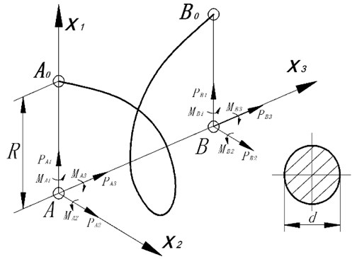
The stiffness matrix of SCFE is dimensionality 12×12, and it can be determined by solving the linear boundary value problems 12 times using the differential equations system [1]. The numerical integration of the system has been carried out using procedure NDSolve in computer package Wolfram Mathematica.
Columns of the matrix are formed as follows. All degrees of freedom SCFE except one are recorded, and the remaining degree of freedom is defined by the unit displacement. Using the kinematics equations of displacements and rotations, the nodes of SCFE A and B are transferred to the edge of helix A0 and B0. After solving the linear boundary value problem of internal forces and moments according to the rules of statics, the nodes are transferred back from points A0 and B0 to points A and B. By deciding these boundary value problems 12 times, we can obtain all the 144 elements of the stiffness matrix. Thus, we can also find the shape functions for each degree of freedom. Note that is the displacement vector function of node, which is located on the axis of the coil and has a single degree of freedom.
In this way, the elements of mass matrix can be calculated by:
where is the shape function of number , is the total length of the helix, and is the cross-sectional area of the wire.
The obtained matrix and of SCFE can be used to construct the lumped stiffness matrix , the lumped mass matrix and form the model of the spring. The frequencies and modes of free vibration can be determined by the traditional homogeneous system [7]:
where is the desired natural frequency and is the unknown vector displacement (waveform).
Actually, the procedure Eigensystem of package Wolfram Mathematica can be used to determine the frequencies and mode shapes of the matrix , which is designed to calculate the eigenvalues and eigenvectors of matrices.
The simulation of the coil spring is with the following initial parameters: external loads and moments = 0, = 0; elastic module of the material = 2∙1011 Pa; Poisson’s ratio = 0.3; density of the spring material = 8000 kg/m3; radius of the coil = 13.25∙10-3 m; wire diameter = 2.6∙10-3 m; helix angle = 3.35°; number of turns = 38.
Comparisons of the experimental results for the first to the fourth natural frequencies are shown in Table 1.
Table 1Comparisons with the results of the experimental natural frequencies p
Frequency number | Calculation, rad/s | Experiment, rad/s | Error |
1-order | 115.3 | 115.2 | 0.09 % |
2-order | 225.0 | 213.6 | 5.34 % |
3-order | 256.5 | 248.2 | 3.34 % |
4-order | 292.0 | 293.2 | 0.41 % |
3. Investigation the impact on the natural frequency of the coil spring with tension and compression
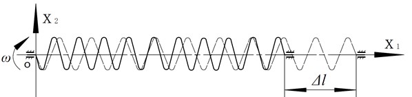
The experiments are performed to determine the frequency and the shape of natural oscillations of the coil spring under the available initial deformations. In order to simulate the operation of the spring mechanism, the experiment platform is designed and constructed in Fig. 2, and it can allow the static and dynamic tests of the coil spring.
The stand allows spring grippers to set the arbitrary position in the base plane. The first gripper has one degree of freedom in the base plane of the stand-rotational. The second gripper has two degrees of freedom, i.e., the translational degree of freedom and the rotational.
Fig. 2Dynamic schemes of the experimental setup
In dynamic tests, as shown in Fig. 3, the spring is mounted on a stand and rotated, which gradually increases the angular velocity until the resonance occurs. The instrument stroboscope ST 4913 can be used to determine the frequency of rotation. In order to facilitate the measurement, a white label is added on the outer surface of the rotating gripper. The frequency measurement is carried out when the outbreak of stroboscope and the white label synchronization are abserved. Due to the stroboscopic effect, we can observe the visual and photography shapes. We need to repeat experiments until they give different initial deformations, which are changed from –20 mm to +40mm.
Fig. 3Experimental setups

a) stroboscope (ST 4913)
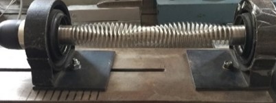
b) Experimental platform

c) Transformer (TEC15)
To calculate the dynamic behavior, the spring can be performed by SCFE, which improves computational efficiency compared with the conventional rod-FE. The CR configuration of each individual element is obtained as a rigid body motion of the element base configuration. Since the large displacement of nodes [3-5] could lead to the complex nonlinear system, the CR approach can be adopted to determine the stiffness and mass matrix of spring with initial deformations. The matrix of the spring is changed due to the different initial deformations. In particular, the algorithm described in this article does not consider a possible contacting turn. It is known that such contacts lead to the extreme complexity. All elements of the changing stiffness matrix can be obtained by:
where is the components tangent stiffness matrix, and are the generalized displacement of nodes, and is the generalized strain energy which can be determined by CR approach. The changing mass matrix can be determined as follows:
where is the initial mass matrix and [L] is the rotation matrix.
Fig. 4Comparison of calculation and experiment for the natural frequencies from the 1st to 4th order
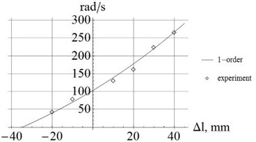
a) 1-order frequency
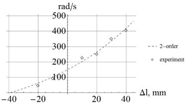
b) 2-order frequency
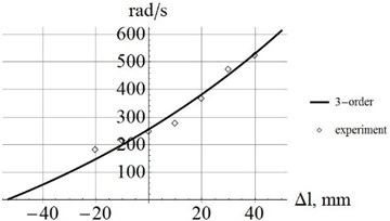
c) 3-order frequency
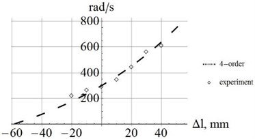
d) 4-order frequency
The detailed explanations and calculations of the CR approach are introduced in [4-5].
From Eqs. (6), (7), we can obtain the changing stiffness matrices and mass matrices, calculate and confirm the natural frequency of the spring. Subsequently, all the curves and experimental data are shown as the following graphics in Fig. 4.
As shown in Fig. 4, it is clear that when the initial deformation increases, the natural frequencies of the spring from the 1st to the 4th order also increase. The intersections of the curves and axes lines are (–35mm, 0); (–39mm, 0); (–46mm, 0); (–57mm, 0), and they are the values of when the natural frequencies of spring become zero.
Table 2Comparing the results of calculation and experimentation with initial deformations
Initial deformation mm | Calculation, rad/s | (Experiment), rad/s | |||||||
Error, % | |||||||||
1-order | 2-order | 3-order | 4-order | ||||||
+40 mm | 260.4 | (266.7) | 391.8 | (405.3) | 517.9 | (524.6) | 616.4 | (612.1) | |
2.36 % | 3.33 % | 1.28 % | 0.70 % | ||||||
+30 mm | 226.8 | (224.9) | 371.3 | (371.4) | 451.1 | (471.3) | 587.4 | (581.1) | |
0.84 % | 0.03 % | 4.29 % | 1.08 % | ||||||
+20 mm | 157.7 | (160.1) | 256.7 | (252.6) | 347.8 | (368.2) | 450.2 | (446.1) | |
1.50 % | 1.62 % | 5.54 % | 0.92 % | ||||||
+10 mm | 135.9 | (130.2) | 229.3 | (226.8) | 265.4 | (261.7) | 330.8 | (341.2) | |
4.38 % | 1.10 % | 2.03 % | 3.04 % | ||||||
–10 mm | 82.7 | (80.1) | 89.7 | (91.7) | 224.9 | (215.6) | 258.7 | (264.5) | |
3.24 % | 2.18 % | 4.31 % | 2.19 % | ||||||
–20 mm | 41.4 | (42.5) | 42.9 | (45.2) | 191.1 | (195.7) | 225.3 | (229.3) | |
2.59 % | 5.09 % | 2.35 % | 1.74 % | ||||||
This table shows that the experimental results of natural frequencies are quite satisfactory. The maximum error is less than 5.54 %.
4. Conclusions
Designing single coil finite element of spring SCFE, with the numerical integration of differential equations Kirchhoff-Clebsch, we can significantly (approximately 20 times) reduce the dimension of the finite element spring model.
The proposed SCFE provides the equation system a much better condition than the traditional finite element. When it is built, the stiffness of the cross section in tensile - compression can be adopted infinite, since the traditional rod-FE technique is impossible.
Comparisons of experimental results for the 1th to 4th order natural frequencies show good accuracy of SCFE when provided initial deformations.
References
-
Badikov R. N. Settlement and Experimental Study of Stress-Strain State and the Resonant Modes of Rotation of Helical Springs in Spring Mechanisms. Candidate Technological Sciences Dissertation, Moscow, 2009.
-
Thomas J. R. Hughes The Finite Element Method Linear Statics and Dynamic Finite Element Analysis. Prentice-Hall, Inc., Englewood Cliffs, New Jersey, 1987, p. 803.
-
Felippa C. A. A Systematic Approach to the Element-Independent Corotational Dynamics of Finite Elements. Technical Report CU-CAS-00-03, Center for Aerospace Structures, 2000, p. 42.
-
Felippa C. A., Haugen B. Unified formulation of small-strain corotational finite elements: I. Theory. Computer Methods in Applied Mechanics and Engineering, Vol. 194, Issues 21-24, 2005, p. 2285-2335.
-
Sorokin F. D. Vector-matrix description of large rotations in the development of finite element mechanical systems. International Scientific School for Youth “Computer Technology Analysis of Engineering Problems of Mechanics”, 2009.
-
Yeliseyev V. V., Zinovieva T. V. Mechanics of Thin-Walled Structures Theory of Rods. St. Petersburg, 2008, p. 95.
-
Douglas T. Structural Dynamics and Vibration in Practice. Elsevier, Amsterdam, 2008, p. 420.
About this article
