Abstract
The flow around a bluff body is a classical problem in the field of fluid mechanics, and its flow mechanism has obvious engineering application value. Numerical simulation is an effective means to solve the problem of flow around bluff body. In recent years, as a new numerical method, lattice Boltzmann method has been more and more concerned and applied in the simulation of complex boundary. Thus, the lattice Boltzmann method is suitable for simulating the flow around bluff body. In this paper, under different Reynolds numbers, numerical simulation is carried out of flow around a square cylinder based on lattice Boltzmann method. And the effect of Reynolds number on the flow around a bluff body is summarized.
1. Introduction
The flow around a bluff body [1] exists widely in the field of construction, transportation and other research because the fluid will produce a large range of separation on the surface of bluff body and form a broad wake with vortex shedding phenomenon, which makes it complex to simulate the turbulent field around bluff body with a simple geometric boundary [2]. In recent years, the lattice Boltzmann method has become a new numerical simulation method, which is suitable for simulating the flow around bluff body. The key of lattice Boltzmann method is to determine the fluid motion distribution function and boundary conditions.
The solution of viscous fluid is not only related to the boundary conditions, but also to the Reynolds number. The smaller the Reynolds number is, the more significant the influence of viscous force is. While the bigger the Reynolds number is, the more significant the influence of inertia force is. When Reynolds number [3, 4] is small, viscous effects are important in the whole flow field. On the contrary, when Reynolds number is high, the effect of fluid viscosity on the flow around a body is important only in the wake of the boundary layer and the rear end of the object. When inertia force and viscous force play an important role in the flow, in order to make the two flow fields with similar geometric satisfy the similar dynamic conditions, the equal Reynolds number of the model and the object must be guaranteed. Therefore, in this paper, we simulate flow around a square cylinder at different Reynolds numbers based on lattice Boltzmann method and demonstrate that BGK-LBM is suitable for flow simulation around bluff body with small Reynolds number.
2. Reynolds number
In 1883, Reynolds observed the flow of fluid in a circular tube [5]. Then firstly he pointed out that the flow pattern was related to three factors including the diameter of the tube, the viscosity of the fluid and the density of the fluid. Reynolds number () indicates the similarity criterion of the viscous effect in fluid mechanics ,
where and are fluid density and kinematic viscosity coefficient respectively, and are characteristic velocity and characteristic length of flow field respectively. Re is physically expressed as the ratio of inertia force and viscous force. As for outflow problem, and are decided on stream velocity far ahead and main dimensions of objects. But as for inner flow problem, they are determined by the average velocity and the diameter of the tube. When the of two geometrically similar flow field is equal, the ratio of the inertia force and viscous force is equal.
When Re is small, the effect of viscous force on the flow field is larger than that of inertia force. The disturbance of flow velocity in flow field will decrease due to viscous force resulting that the fluid flow is stable in the form of laminar flow. Conversely, when is high [6], the effect of inertia force on the flow field is larger than that of viscous force. And the fluid flow is somehow unstable. The micro change of the flow velocity is easy to develop and strengthen. It’s also easy to form a disordered and irregular turbulent flow field.
3. The Lattice Boltzmann method
The Lattice Boltzmann method [7-9] (LBM) is one of the most important achievements in recent 20 years of computational fluid mechanics and different from the traditional numerical methods [6] for fluid calculation and modeling method describing the movement of the molecule. LBM regards the fluid as discrete system composed of a large number of mesoscopic particle. According to the movement characteristics of the particle, a simplified LB equation is established to calculate the evolution of particle distribution function.
LBE [11] is an integro-partial differential equation, so one of the difficulties in solving LBE is the complexity of the collision integral. In order to simplify the solving process, a collision function model with a simple operator instead of collision was proposed by Bhatnagar, Gross and Krook in 1954. LBE is a special discrete form of Boltzmann-BGK equation including discrete velocity, discrete time and space discretization.
The lattice Boltzmann evolution equation of the single relaxation time is:
where , , , are the relaxation factor, discrete velocity, particle distribution function and equilibrium distribution function respectively.
In 1992, professors including Qian proposed the model DnQb [11] n and b refer to space dimension and discrete velocity respectively) and the equilibrium distribution function is:
where is sound velocity of the grid and is weight coefficient. The two parameters decide that the rage of lattices depends on the selecting of in discrete velocity model.
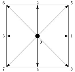
In this paper, we adopted D2Q9 model (shown as Fig. 1).
Fig. 1D2Q9 model
, :
Weight coefficient and sound velocity of lattices are as follows:
In the formula, is velocity of grid. and are grid length and time step respectively.
The macroscopic velocity and momentum of fluid are:
The relationship between the fluid viscosity coefficient and the relaxation factor of the model is:
Generally, the calculation process of LBE is as follows:
(1) Initialize the distribution function:
(2) Perform collision at :
(3) Perform migration:
(4) Calculate macroscopic thermodynamic quantities:
Repeat steps (2)-(4) until the terminal conditions are met.
In LBM, the accurate simulation of boundary conditions [12-14] is an important and crucial problem, because the boundary conditions are not easy to determine, which needs to confirm the distribution function of the boundary. At present, the types of boundary of LBM can be divided into heuristic schemes, dynamic schemes and interpolation/extrapolation schemes. According to the type of boundary condition, it also can be divided into the velocity boundary and the pressure boundary. Additionally, there are some special artificial boundaries, such as the entrance, exit, infinity, symmetry, etc.
4. Flow simulation around a square cylinder at different Reynolds number
The solution of viscous fluid is not only related to the boundary conditions, but also to . We choose a rectangle with 400 meters’ length and 45 meters’ width as the computational domain. We suppose the wind velocity is 5 m/s and the Reynolds number is 20. We chose the standard rebounded scheme as the surface free slip boundary and dealt with the flow inlet velocity boundary and the exit constant pressure boundary by the non-equilibrium rebounded scheme. As follows, we selected different to simulate the flow.
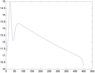
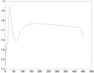
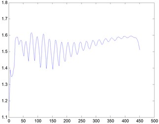
1) 20. The barrier is a rectangular cylinder [15] of 5 m×5 m placed at 20 meters’ away from the entrance. When the Reynolds number is 20, we obtain the streamline, three-dimensional graph and curve graph of maximum speed in a line by use of the MATLAB after 40000 steps of the calculation, as shown in Figs. 2-4.
Fig. 2Streamline, Re= 20
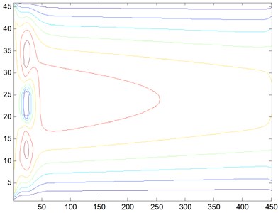
Fig. 33D graph, Re= 20
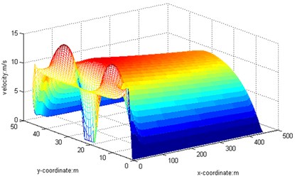
Fig. 4Curve graph, Re= 20
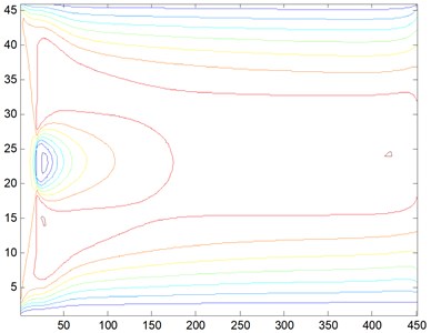
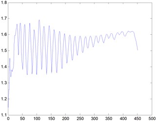
2) 100. The barrier is a rectangular cylinderof 5 m×5 m placed at 20 meters’ away from the entrance. When the Reynolds number is 100, we obtain the streamline, three-dimensional graph and curve graph of maximum speed in a line by use of the MATLAB after 40000 steps of the calculation, as shown in Figs. 5-7.
Fig. 5Streamline, Re= 100
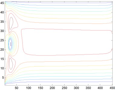
Fig. 63D graph, Re= 100
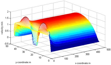
Fig. 7Curve graph, Re= 100
3) 500. The barrier is a rectangular cylinderof 5 m×5 m placed at 20 meters’ away from the entrance. When the Reynolds number is 500, we obtain the streamline, three-dimensional graph and curve graph of maximum speed in a line by use of the MATLAB after 40000 steps of the calculation, as shown in Figs. 8-10.
Fig. 8Streamline, Re= 500
4) 1000. The barrier is a rectangular cylinderof 5 m×5 m placed at 20 meters’ away from the entrance. When the Reynolds number is 1000, we obtain the streamline, three-dimensional graph and curve graph of maximum speed in a line by use of the MATLAB after 40000 steps of the calculation, as shown in Figs. 11-13.
Fig. 93D graph, Re= 500
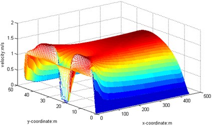
Fig. 10Curve graph, Re= 500
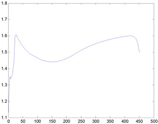
Fig. 11Streamline, Re= 1000
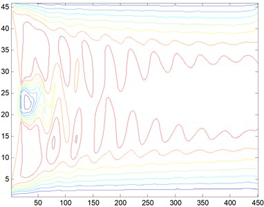
Fig. 123D graph, Re= 1000
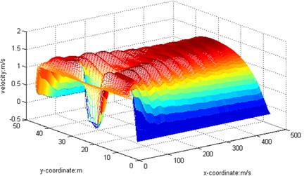
Fig. 13Curve graph, Re= 1000
5) 2000. The barrier is a rectangular cylinderof 5 m×5 m placed at 20 meters’ away from the entrance. When the Reynolds number is 2000, we obtain the streamline, three-dimensional graph and curve graph of maximum speed in a line by use of the MATLAB after 40000 steps of the calculation, as shown in Figs. 14-16.
We can see from the flow around the wake that the variation of the flow field is obvious, and it will gradually tend to be stable after the obstacles. According to Figs. 2-16, we can see that when Re is small, the air velocity of the flow field around the obstacle is larger and it will gradually tend to be stable after the obstacle. However, when Re reaches 1000, apart from big ups and downs of air velocity around the obstacle, the air velocity in flow field after the obstacle is still showing a wave of instability.
Fig. 14Streamline, Re= 2000
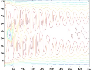
Fig. 153D graph, Re= 2000
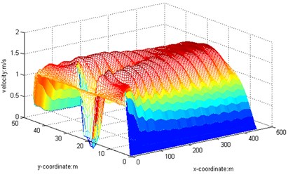
Fig. 16Curve graph, Re= 2000
5. Conclusion
The flow around a bluff body is a classical problem in the field of fluid mechanics. Due to the accuracy of the existing numerical simulation method is low, in this paper; we put forward a numerical simulation method with high accuracy and good stability based on molecular dynamic theory. By using MATLAB to compile calculation program, we carried out the numerical simulation of flow around a square cylinder at different Re and we obtain the streamline, three-dimensional graph and curve graph of maximum speed in a line to study the characteristics of flow around a bluff body. Through the analysis, the following conclusions are drawn: under the conditions of small Re, the variation of flow field around the bluff body is more obvious and it will gradually tend to be stable, which is consistent with the actual theory. With the increase of Re, the air velocity in flow field after the obstacle is still showing a wave of instability. Therefore, BGK-LBM is suitable for the flow simulation of bluff body under small Reynolds numbers.
References
-
Prosser T. Daniel, Smith J. Marilyn Characterization of flow around rectangular bluff bodies at angle of attack. Physics Letters A, Vol. 376, 2012, p. 3204-3207.
-
Haghighi Erfan, Or Dani Interactions of bluff-body obstacles with turbulent airflows affecting evaporative fluxes from porous surfaces. Journal of Hydrology, Vol. 530, 2015, p. 103-116.
-
Li Hong, Jin Xiang-hong, Deng Hai-shun, Lai Yong-bin Experimental investigation on the outlet flow field structure and the influence of Reynolds number on the outlet flow field for a bladeless fan. Applied Thermal Engineering, Vol. 100, 2016, p. 972-978.
-
Bayon Arnau, Valero Daniel, Garcia-Bartual Rafael, Valles-Moran Francisco Jose, Lopez-Jimenez P. Amparo Performance assessment of OpenFOAM and FLOW-3D in the numerical modeling of a low Reynolds number hydraulic jump. Environmental Modeling and Software, Vol. 80, 2016, p. 322-335.
-
Crespi-Llorens D., Vicente P., Viedma A. Generalized Reynolds number and viscosity definitions for non-Newtonian fluid flow in ducts of non-uniform cross-section. Experimental Thermal and Fluid Science, Vol. 64, 2015, p. 125-133.
-
Bernardini Matteo, Modesti Davide, Pirozzoli Sergio On the suitability of the immersed boundary method for the simulation of high-Reynolds-number separated turbulent flow. Computers and Fluids, Vol. 130, 2016, p. 84-93.
-
Shan Xiaowen The mathematical structure of the lattices of the lattice Boltzmann method. Journal of Computational Science, 2016, (in press).
-
Tao Shi, Hu Junjie, Guo Zhaoli An investigation on momentum exchange methods and refilling algorithms for lattice Boltzmann simulation of particulate flows. Computers and Fluids, Vol. 133, 2016, p. 1-14.
-
Raman Kuppa Ashoke, Jaiman Rajeev K., Lee Thong-See, Low Hong-Tong Lattice Boltzmann study on the dynamics of successive droplets impact on a s solid surface. Chemical Engineering Science, Vol. 145, 2016, p. 181-195.
-
Zhang Jianying, Yan Guangwu Simulations of the fusion of necklace-ring pattern in the complex Ginzburg-Landau equation by lattice Boltzmann method. Communications in Nonlinear Science and Numerical Simulation, Vol. 33, 2016, p. 43-56.
-
Feng Yongliang, Sagaut Pierre, Tao Wen-Quan A compressive lattice Boltzmann finite volume model for high subsonic and transonic flows on regular lattices. Computers and Structures, Vol. 131, 2016, p. 45-55.
-
Wang Y., Shu C., Teo C. J., et al. An efficient immersed boundary-lattice Boltzmann flux solver for simulation of 3D incompressible flows with complex geometry. Computers and Fluids, Vol. 124, Issue 2, 2016, p. 54-66.
-
Li Zhe, Favier Julien, D’Ortona Umberto, Poncet Sebastien An immersed boundary-lattice Boltzmann method for single- and multi-component fluid flows. Journal of Computational Physics, Vol. 304, 2016, p. 424-440.
-
Delouei Amiri A., Nazari M., Kayhaini M. H., Ahmadi G. A non-Newtonian direct numerical study for stationary and moving objects with various shapes: an immersed boundary-lattice Boltzmann approach. Journal of Aerosol Science, Vol. 93, 2016, p. 45-62.
-
Nguyen Vinh-Tan, Nguyen Hoa Hug Detached eddy simulations of flow induced vibrations of circular cylinders at high Reynolds numbers. Journal of Fluids and Structures, Vol. 63, 2016, p. 103-119.
About this article
This paper is supported by the National Natural Science Foundation of China (11472248).
