Nonlocal thermoelastic vibrations for variable thermal conductivity nanobeams due to harmonically varying heat

1. Introduction

Nanotechnology has wide applications, which include the fabrication of engineering structures at nanoscale enabling production of materials with revolution properties and devices with enhanced functionality. One of these structures is nanobeams, which have been used widely in systems and devices such as atomic force microscope, nanowires, nano-actuators and nano-probes (Chakraverty [1]). The thermoelastic solutions may be completely incorrect with the ignoring of small-scale effects in sensitive nano-designing fields. Since mechanical behavior of nanostructures could not be predicted accurately by classical continuum theories. So, nonlocal continuum theories have been proposed to include the small scale effect in vibration and buckling of nanobeams.

In 1972, Eringen [2] proposed a theory, called nonlocal continuum mechanics, in an effort to deal with the small-scale structure problems. In the classical (local) continuum elasticity, the material particles are assumed to be continuously distributed and the stress tensor at a reference point is uniquely determined by the strain mechanics is based on the constitutive functionals being functional of the past deformation histories of all material points of the body concerned. The small length scale effects are counted by incorporating the internal characteristic length such as the length of the C-C bond into the constitutive relationship. Solutions from various problems support this theory (Eringen [2, 3]; Eringen and Edelen [4]). For examples, the dispersion curves by the nonlocal model are in excellent agreement with those by the Born-Karman theory of lattice dynamics; the dislocation core and cohesive stress predicted by the nonlocal theory are close to those known in the physics of solids (Eringen [3]; Eringen and Edelen [4]). Zhang et al. [5] and Lu et al. [6] determined the values of scaling effect parameter experimentally and they used these values in vibration and buckling problems of nanostructures. In addition, the first author and his colleagues [7-10] have recently discussed the behavior of nanobeam in the context of a nonlocal thermoelasticity theory.

The present paper investigates the coupling effect (Lord and Shulman [11]; Green and Lindsay [12]; Green and Naghdi [13]) between temperature and strain rate in nanobeams with variable thermal conductivity (Berman [14]) based on the nonlocal dual-phase-lag model. The solution for the generalized thermoelastic vibration of a nanobeam subjected to time-dependent temperature is developed. The Laplace transform method is used to determine the lateral vibration, temperature, displacement, and bending moment of the nanobeam. The effects of nonlocal parameter, phase-lags, angular frequency of thermal vibration and the variability thermal conductivity parameter are investigated.

2. Mathematical modeling and basic equations

Let us consider a homogenous isotropic thermoelastic solid in Cartesian coordinate systems $Oxyz$ initially un-deformed and at uniform temperature $T_0\text{.}$ The modified of classical thermoelasticity model is given by Tzou theory (Tzou [15-17]) in which the Fourier law is replaced by an approximation of the equation:

where $\mathbf{q}$ denotes the heat flux vector, $K$ denotes the thermal conductivity, $\theta =T-T_0$ is the temperature increment of the resonator, in which $T_0$ is the environmental temperature, $T(x,z,t)$ denotes the temperature distribution, ${\tau }_{\theta }$ and ${\tau }_q$ represent the delay times. The delay time ${\tau }_{\theta }$ is said to be the phase-lag of temperature gradient and ${\tau }_q$ is the phase-lag of heat flux. The above equation may be approximated as:

where $0\le {\tau }_{\theta }<{\tau }_q$. The heat conduction equation corresponding to the dual-phase-lag model proposed by Tzou [15-17] in this case takes the form:

where $C_E$ denotes the specific heat per unit mass at constant strain, $e=\partial u/\partial x+\partial v/\partial y+\partial w/\partial z$ is the volumetric strain, $\gamma =E{\alpha }_T/(1-2\nu )$ in which ${\alpha }_T$ is the thermal expansion coefficient, $E$ is Young’s modulus and $\nu$ is Poisson’s ratio, $\rho$ is the material density of the medium, and $Q$ is the heat source.

The general nonlocal constitutive equations for a nanobeam can be written as [3]:

where ${\sigma }_{kl}$ denotes the nonlocal stress tensor, ${\tau }_{kl}$ denotes the classical (Cauchy) or local stress tensor and ${\nabla }^2$ is the Laplacian. The parameter $a$ is the internal characteristic length, $l$ is the external characteristic length (e.g., crack length, wave-length), and $e_0$ is a constant appropriate to each material.

Eq. (3) describes the non-local coupled dynamical thermoelasticity theory, the generalized thermoelasticity theories proposed by Lord and Shulman [11], and dual-phase-lag model (Tzou [15-17]) for different sets of values of phase-lags parameters ${\tau }_q$ and ${\tau }_{\theta }$ as follows:

• The nonlocal coupled thermoelasticity (CTE) theory results from Eq. (3) by taking ${\tau }_{\theta }={\tau }_q=\text{0}$.

• The nonlocal generalized theory with one relaxation time (LS theory) can be obtained when ${\tau }_{\theta }=\mathrm{}$0, ${\tau }_q={\tau }_0$ (${\tau }_0$ is the relaxation time).

• The nonlocal generalized theory with two dual-phase-lags (DPL) theory is given by setting ${\tau }_q\ge {\tau }_{\theta }>\text{0}$.

It can be seen that the corresponding local thermoelasticity is recovered by putting $a{e}_0=\text{0}$ in the above equations.

3. Formulation of the problem

Let us consider small flexural deflections of a thin elastic nanobeam with dimensions of length $(0\le x\le L)$, width $b$$(-b/2\le y\le +b/2)$ and thickness $h$$(-h/2\le z\le +h/2)$, as shown in Fig. 1. We define the $x$-axis along the axis of the beam and the $y$- and $z$-axes correspond to the width and thickness, respectively.

Fig. 1Schematic diagram of the nanobeam

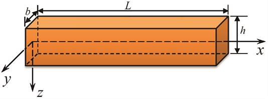
In equilibrium, the beam is unstrained, unstressed and at temperature $T_0$ everywhere. The displacements according to Euler-Bernoulli beam theory are given by:

where $w$ is the lateral deflection. It is to be noted that, the nonlocal theory assumes that stress at a point depends not only on the strain at that point but also on strains at all other points of the body. So, the one-dimensional constitutive equation gives the uniaxial tensile stress only, according to the differential form of the nonlocal constitutive relation proposed by Eringen [2, 3], as:

where $\mathrm{\xi }=(a{e}_0{)}^2$ is the nonlocal parameter. The flexure moment of the cross-section is given by:

where $EI$ is the flexural rigidity of the beam in which $I=b{h}^3/\text{12}$ denotes the inertia moment of the cross-section and $M_T$ is the thermal moment:

The equation of motion is given by:

where $A=bh$ denotes the cross-section area. Substituting Eq. (7) into Eq. (9), the equation of motion becomes:

In case of the nonlocal theory, the bending moment can be written as:

It is exactly seen that when the parameter $\xi$ is set identically to zero, the local Euler-Bernoulli beam theory will be obtained.

4. Temperature-dependent thermal conductivity

Generally, the assumption that the solid body is thermosensitivity (the thermal properties of the material vary with temperature) leads to a nonlinear heat conduction problem. The exact solution of such problem can be found by assuming the material to be (simply nonlinear) meaning that the thermal conductivity $K$ and specific heat $C_E$ depend on the temperature, but thermal diffusivity $k$ is assumed be constant.

The thermal conductivity $K$ is assumed to vary linearly with temperature according to [14]:

where $K_0$ is the thermal conductivity at ambient temperature $T_0$ and $K_1$ is the slope of the thermal conductivity-temperature curve divided by the intercept $K_0$. Now, we will consider the Kirchhoff transformation [14]:

where $\psi$ is a new function expressing the heat conduction. By substituting Eq. (12) in Eq. (13), we get:

From Eq. (13), it follows that:

After substituting Eqs. (15) and (16) into Eq. (3), the new form of the general heat equation of solids with temperature-dependent thermal conductivity is obtained by the form:

where $\rho C_E=K/k$. Substituting the Euler-Bernoulli assumption given in Eq. (5) into Eq. (17) gives the thermal conduction equation for the beam without the heat source $(Q=\text{0})$, as:

For a nanobeam, assuming that the temperature increment varies sinusoidally along the thickness direction. That is:

Using Eqs. (8), (12) and (15), Eq. (10) will be in the form:

where $c=\sqrt{E/\rho }$ denotes the speed of propagation of isothermal elastic waves. Since $\theta =T-T_0$ such that $\left|\theta /T_0\right|\ll 1$, then for linearity, Eq. (20) will be:

Now, multiplying Eq. (18) by means of $12z/h^3$ and integrating it with respect to $z$ through the beam thickness from $-h/2$ to $h/2$, yields:

The preceding governing equations can be put in non-dimensional forms by using the following dimensionless parameters:

So, the governing equations, and the bending and constitutive equations in non-dimensional forms are simplified as (dropping the primes for convenience):

where:

5. Initial and boundary conditions

In order to solve the problem, both the initial and boundary conditions should be considered. The initial conditions of the problem are taken as:

These conditions are supplemented by considering the two ends of the nanobeam are subjected to the following boundary conditions:

Let us also consider the micro-beam is loaded thermally by a harmonically varying incidents into the surface of the nanobeam $x=\text{0}$:

where $\omega$ is the angular frequency of thermal vibration ($\omega =0$ for a thermal shock problem) and ${\mathrm{\Theta }}_0$ is constant. Using Eqs. (13) and (19), then one gets:

Assuming that the boundary $x=L$ is thermally insulated, this means that the following relation will be satisfied:

Using Eqs. (14) and (19), then one gets:

6. Solution in the Laplace transform domain

The closed form solution of the governing and constitutive equations may be possible by adapting the Laplace transformation method. Applying the Laplace transform to Eqs. (24)-(26), one gets the field equations in the Laplace transform space as:

where an over bar symbol denotes its Laplace transform, $s$ denotes the Laplace transform parameter and:

Elimination $\stackrel{-}{\mathrm{\Psi }}$ or $\stackrel{-}{w}$ from Eqs. (34) and (35) gives the following differential equation for both $\stackrel{-}{w}$ or $\stackrel{-}{\mathrm{\Psi }}$:

where the coefficients $A$, $B$ and $C$ are given by:

Introducing $m_i$$(i=\text{1,}\text{2,}\text{3})$ into Eq. (38), one gets:

where $D=d/dx$ and $m_1^2$, $m_2^2$ and $m_3^2$ are the roots of the characteristic equation:

These roots are given by:

where:

The solution of the governing equations in the Laplace transformation domain can be represented as:

where $C_i$ and $F_i$ are parameters depending on $s$. The compatibility between Eqs. (35) and (44), gives:

Then, the axial displacement after using Eqs. (5) and (44) takes the form:

In addition, the strain will be:

After using Laplace transform, the boundary conditions take the forms:

Substituting Eqs. (44) into the above boundary conditions, one obtains six linear equations in the matrix form as:

After solving the above equations, we have the values of the constants $C_i$, $i=\mathrm{}$1, 2,..., 6 whose solution complete the solution of the problem in the Laplace transform domain. Hence, we obtain the expressions for the non-dimensional lateral vibration, displacement, the stress and other physical quantities of the medium.

After obtaining $\stackrel{-}{\mathrm{\Psi }}$, the temperature increment $\stackrel{-}{\theta }$ can be obtained by solving Eq. (14) and using Eq. (19) to give:

Then, the bending moment $M$ given in Eq. (36) in the Laplace domain with the aid of the Eqs. (44) and (45), become:

7. Inversion of the Laplace transforms

In order to invert the Laplace transform in the above equations, we adopt a numerical inversion method based on a Fourier series expansion. Durbin [18] derived the approximation formula:

where $\stackrel{-}{f}\left(s\right)$ being the Laplace transform. It is known that $\mathrm{R}\mathrm{e}\left[\stackrel{-}{f}\right(s+2in\pi /t_1\left)\right]$ and $\mathrm{I}\mathrm{m}\left[\stackrel{-}{f}\right(s+2in\pi /t_1\left)\right]$ tend to $0$ when $n$ tends to infinity. To apply efficiently each of the above mentioned procedures, one would have first to find, in each case, the value of $n$ after which $\stackrel{-}{f}(s+2in\pi /t_1)$ decreases monotonically to 0. This is virtually impossible for the very complicated $\stackrel{-}{f}\left(s\right)$. So, the real and imaginary part of $\stackrel{-}{f}\left(s\right)$ are evaluated together through a complex, single precision arithmetic subroutine, but are converted into double precision constants for the summation up to NSUM; the results are then turned back to single precision expressions. Thus, one avoids time and storage consuming systematic double precision computation; NSUM can be determined by the convergence criterion:

It should be noted that a good choice of the free parameters $n$ and $s{t}_1$ is not only important for the accuracy of the results, but also for the application of the Korrecktur method and the methods for the acceleration of convergence. We found that $s{t}_1=\text{5}$ to 10 give good results for NSUM ranging from 50 to 5000. The values of all parameters in Eq. (39) are defined as $t_1=\text{20,}$$s=\text{0.25}$ and $N=\text{1000}$ in this paper (Durbin [18]).

Fig. 2Distribution of the field quantities through the axial direction for different theories of thermoelasticity

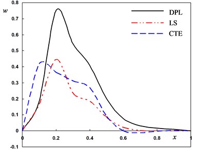
a) The deflection

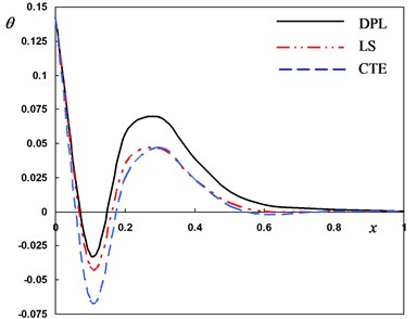
b) The temperature

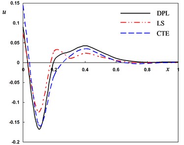
c) The radial displacement

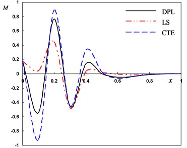
d) The bending moment

8. Numerical results

In terms of the Riemann-sum approximation defined in Eq. (52), numerical Laplace inversion is performed to obtain the non-dimensional lateral vibration, temperature, displacement and bending moment in the nanobeam. In the present work, the thermoelastic coupling effect is analyzed by considering a beam made of silicon. The material parameters are given as:

The aspect ratios of the beam are fixed as $L/h=\text{10}$ and $b/h=\text{0.5}$. The figures were prepared by using the non-dimensional variables which are defined in Eq. (14) for a wide range of beam length when $L=\text{1}$, $z=h/6$ and $t=\mathrm{}$0.12 sec.

Numerical calculations are carried out for four cases. In the first case the non-dimensional lateral vibration, temperature, displacement and bending moment with different phase-lags are investigated when the pulse-width and nonlocal parameter remain constants $\text{(}\omega =$ 5, $\stackrel{-}{\xi }=1\text{)}$. The graphs in Fig. 2(a)-(d) represent the curves predicted by three different theories of thermoelasticity obtained as special cases of the present dual-phase-lag model. The computations are performed for various values of the parameters ${\tau }_q$ and ${\tau }_{\theta }$ to obtain the coupled theory (CTE) (${\tau }_q={\tau }_{\theta }=0$), the Lord and Shulman (LS) theory $\text{(}{\tau }_{\theta }=\text{0}$ and ${\tau }_q=\text{0.}\text{0}\text{2)}$ and the generalized theory of thermoelasticity proposed by Tzou (DPL) (${\tau }_q=\text{0.}\text{0}\text{2}$ and ${\tau }_{\theta }=\text{0.01}$).

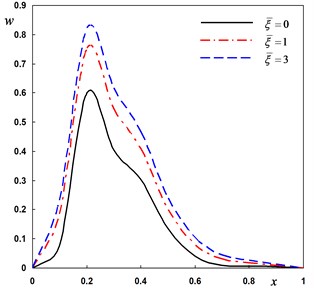
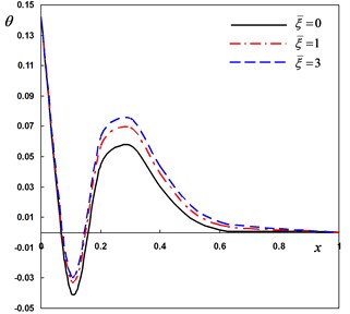
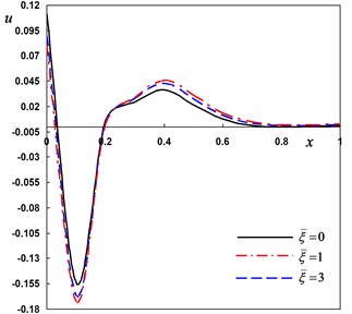
Fig. 3Distribution of the field quantities through the axial direction for various thermal conductivity parameters

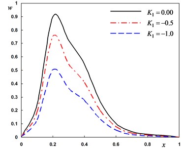
a) The deflection

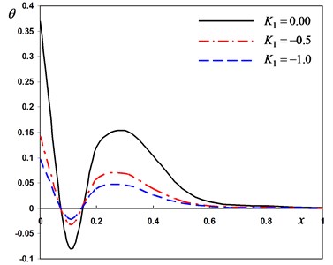
b) The temperature

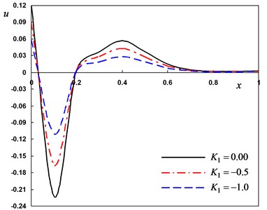
c) The radial displacement

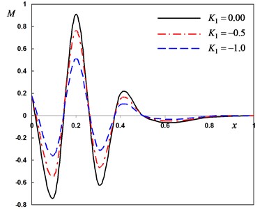
d) The bending moment

Fig. 2(a) depicts the distribution of the lateral vibration $w$ which always begins and ends at the zero values (i.e. vanishes) and satisfies the boundary condition at $x=\text{0}\text{,}L$. In the context of three theories, the values of $w$ starts increasing to maximum amplitudes in the range $\text{0}\le x<\text{0.3,}$ thereafter it moves in the direction of wave propagation. The behavior of DPL model may be differ than those of other two theories.

It is observed from Fig. 2(b) that the temperature $\theta$ decreases as the distance $x$ increases to move in the direction of wave propagation. The temperature of DPL model may be similar than those of other models.

Fig. 2(c) shows that the values of the displacement $u$ start decreasing in the range $\text{0}\le x\le \text{0.1,}$ thereafter increasing to maximum amplitudes in the range $\text{0.1}\le x\le \text{0.4}$. The displacement moves directly in the direction of wave propagation in the range $\text{0.4}\le x\le \text{1}$.

In Fig. 2(d), the bending moment is zero when $x=L$ at the boundary of the beam and it attains a stationary maximum value at some positions.

It can be observed that the phase-lags parameters have great effects on the distribution of field quantities. The mechanical distributions indicate that the wave propagates as a wave with finite velocity in medium. The fact that in thermoelasticity theories (DPL, LS, CTE), the waves propagate with finite speeds is evident in all these figures. The behavior of the three theories is generally quite similar.

Fig. 4Distribution of the field quantities through the axial direction for various angular frequencies of thermal vibration

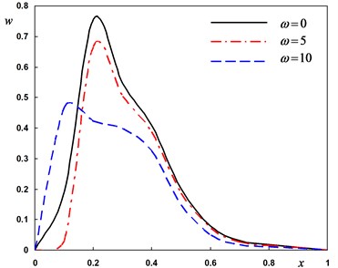
a) The deflection

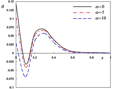
b) The temperature

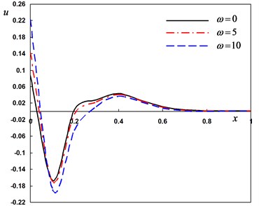
c) The radial displacement

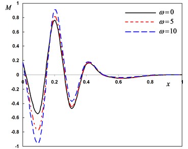
d) The bending moment

In second case, we consider three different values the variability thermal conductivity parameter $K_1$ to discuss the thermosensitivity (the thermal properties of the material vary with temperature). We take $K_1=\mathrm{}$–1, –0.5 for variable thermal conductivity and $K_1=0$ when thermal conductivity is independent of temperature. In this case the angular frequency of thermal vibration $\omega =\text{5}$ and phase-lag of the heat flux ${\tau }_q=\text{0.02}$ and the phase-lag of temperature gradient ${\tau }_{\theta }=\text{0.01}$. From Fig. 3(a)-(d), the parameter $K_1$ has significant effects on all the fields. From Fig. 3(a), 3(c) and 3(d), the lateral vibration $w$, the temperature $\theta$ and bending moment $M$ decreases as the $K_1$ decreases. From Fig. 3(b), it can be found that the displacement $u$ decreases as the parameter $K_1$ value decreases in the range $\text{0}\le x\le \text{0.2}$ and increases in the range $\text{0.2}\le x\le \text{1}$. The medium close to the beam surface suffers from tensile stress, which becomes larger with the time passing. We have noticed from the figures that, the variability thermal conductivity parameter $K_1$ has a significant effect on all the fields, which add an importance to our consideration about the thermal conductivity to be variable. It is clear that the maximum values of occur near the surface $x=\text{0}$ of the beam and its magnitude decreases with the increase of $x$.

Fig. 5Distribution of the field quantities through the axial direction for various nonlocal parameters

a) The deflection

b) The temperature

c) The radial displacement

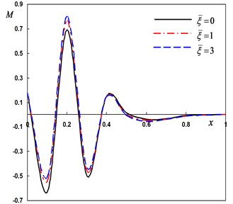
d) The bending moment

In the third case, three different values of the angular frequency of thermal vibration were considered. For thermal shock problem, we put $\omega =\text{0}$ and for harmonically heat $\omega$ is set to $\omega =\text{5,}\text{10}$. In this case the variability thermal conductivity parameter $K_1$ is fixed to –0.5. From Fig. 4 (a)-(d), the values of the lateral vibration, temperature, displacement and bending moment decreases as $\omega$ decreases. These figures illustrate that, the angular frequency parameter $\omega$ has a significant effects on all the fields.

Next, the DPL model is used to investigate the non-dimensional lateral vibration, temperature and displacement for different values of the nonlocal parameter $\stackrel{-}{\xi }$$\text{(}{\tau }_q=\text{0.02,}$${\tau }_{\theta }=\text{0.01,}$$K_1=\mathrm{}$–0.5, $\stackrel{-}{\xi }=\text{1}\text{)}$. The numerical results are obtained and presented graphically in Fig. 5(a)-(d). It is seen that the effect of the nonlocal parameter $\stackrel{-}{\xi }$ on all the studied fields is highly significant.

The last case is to investigate the non-dimensional lateral vibration, temperature and displacement for various values of the nonlocal parameter $\xi =\mathrm{}$10^–7$\stackrel{-}{\xi }$, ($\stackrel{-}{\xi }=\mathrm{}$0, 1, 2) when the pulse width remains constant $\text{(}{\tau }_q=\text{0.02}\text{,}\mathrm{}{\tau }_{\theta }=\text{0.01,}\omega =\text{5,}\mathrm{}z=h/\text{6).}$ It can be seen that the corresponding local thermoelasticity model is recovered by putting $\stackrel{-}{\xi }=0$. The variations of the field variables with various values of the nonlocal parameter are depicted in Fig. 5(a)-(d). Generally, the field variables are very sensitive to the variation of the nonlocal parameter.

9. Conclusions

In this paper, a new model of nonlocal generalized thermoelasticity with dual-phase-lags for the Euler-Bernoulli nanobeam under variable thermal conductivity is constructed. The vibration characteristics of the deflection, temperature, the displacement and the bending moment of nanobeam subjected to harmincally varying heat heating are investigated. The effects of the nonlocal parameter $\stackrel{-}{\xi }$ and the angular frequency of thermal vibration $\mathrm{\omega }$ on the field variables are investigated.

Numerical simulation results yield the following conclusions:

• The variability thermal conductivity parameter has significant effects on the speed of the wave propagation of all the studied fields.

• The dependence of the thermal conductivity on the temperature has a significant effect on thermal and mechanical interactions.

• According to the results shown in all figures, we find that the nonlocal parameter $\stackrel{-}{\xi }$ has significant effects on all the field quantities. On the other hand the thermoelastic stresses, displacement and temperature have a strong dependency on the angular frequency of thermal vibration parameter.

• The dual-phase-lag model of thermoelasticity predicts a finite speed of wave propagation that made the generalized theorem of thermoelasticity more consistent with the physical properties of the material. Also, it was found that the phase lags of the heat flux and temperature gradient ${\tau }_q$ and ${\tau }_{\theta }$ play a significant role on the behavior of all field variables.

• The Lord and Shulman (LS) theory and the classical thermoelasticity theory (CTE) are obtained as special cases of the present model.

• The paper also concludes the governing equation of motion for a nonlocal nanobeam can be formed by replacing the bending moment term in the classical equation of motion with an effective nonlocal bending moment as presented herewith. It is found that the effect of the nonlocal parameter is very pronounced. Finally, this work is expected to be useful to design and analyze the wave propagation properties of nanoscale devices.