Research on fault law of rolling bearing under different fault levels and loads with HHT method

Yongbao, Liu; Qiang, Wang; Shuyong, Liu; Xing, He

Journal of Measurements in Engineering

Browse Journal

Submit article

Published: 30 June 2014

Check for updates

Research on fault law of rolling bearing under different fault levels and loads with HHT method

Liu Yongbao¹

Wang Qiang²

Liu Shuyong³

He Xing⁴

^{1, 2, 3, 4}College of Power Engineering, Naval University of Engineering, WuHan, China

Corresponding Author:

Wang Qiang

Cite the article Download PDF

Downloads 1398

Abstract

Bearing is one of the most important components of rotating machinery. The vibration signals are generally nonlinear and nonstationary while operating. The failed rolling bearing will damage to the machine, or cause a serious loss of property. There are a lot of methods about fault diagnosis of bearing, such as shock pulse method, resonance demodulation. Especially the HHT (Hilbert-Huang Transform) method with the adaptive advantage has gradually become a very promising method to extract the characteristics of nonlinear, nonstationary signal. In this paper the variant energy method was introduced in HHT to reduce the computation of the decomposed signal, which effectively improved the computation, and then an experimental platform was designed and established. The bearing fault categories can be diagnosed correctly in dealing with the vibration signals using this method and the fault law is discovered that the trend of the vibration signal fault characteristic frequency amplitude changes with the load increasing. The bearing failure mechanism provides beneficial reference for further research of nonlinear signal analysis.

1. Introduction

Bearing is one of the most important components of rotating machinery, and it could be an easily damaged one. On account of long-term running or improper assembly, wear and tear fault of mechanical component occurs often in rotating machinery such as steam engine, aircraft engine and gas turbine. Therefore, how to diagnose the bearing is an important task. The vibration signal strongly related to the machine features in general, implies the information of operating conditions. Therefore, the vibration analysis becomes the major technique for diagnosing the faults of bearing, as well as it has motivated many researchers and engineers to study this problem.

The conventional fast Fourier transform (FFT) has difficulty in detecting the weak signs of faults at an early stage. Because of wavelet transform involves the operations of dilation and translation, which lead to a multi-scale analysis of the signal when it is applied to nonlinear and nonstationary time series [1]. Lim and Leong [2] and Inoue et al. [3] utilized wavelet analysis to detect looseness faults of structures. In recent years, the Hilbert-Huang transform (HHT) is becoming a popular tool for processing weak signals, and has been generalized to complicated data analysis in different fields [4, 5]. It is constituted by two parts, i.e. empirical mode decomposition (EMD) and Hilbert Transform. The empirical mode decomposition is capable to decompose the complicated signals into finite number of intrinsic mode functions (IMF), and then dispose the decomposed signals using Hilbert Transform method. By employing the significant test to the IMFs, the contained information of IMFs can be extracted, and the traditional Fourier filtering process is not required. The marginal Hilbert spectra are composed of the IMFs and determined through the Hilbert transform. Finally the features of wear and tear faults can be identified by analyzing the Hilbert spectra. The effectiveness of the proposed method is evaluated by measuring the fault indices among the spectra of different types of wear and tear, which shows that the proposed method can distinguish the similarities among the marginal Hilbert spectrum distributions, and thus the identification of the bearing wear faults of different mechanical components can be achieved.

2. The HHT analysis

When applying the HHT, firstly, the EMD will be carried out to obtain the intrinsic mode functions (IMF) which is a kind of complete, adaptive and almost orthogonal representation for the analyzed signal. Since the IMF is almost monocomponent, it can determine all the instantaneous frequencies from the nonlinear or nonstationary signals. Secondly, the local energy of each instantaneous frequency is derived from the Hilbert Transform.

A thorough theoretical discussion on this definition of frequency was given by Huang et al. (1998). By using EMD together with HT, it is possible to calculate the instantaneous frequency of a nonstationary signal generated by a nonlinear system. This algorithm is considered as one of the most important discovery in the last two centuries [6, 7], and it has been widely used in signal processing. In 2004, P. Flandrin [8] et al. used the EMD algorithm in the broadband noise of the random sequence, a half band filter was realized through it. In 2006 R. C. Sharpley and V. Vatchev had a further research to improve intrinsic mode function of transformation method [9]. In 2008, G. Ring et al. studied the extreme value point location information of each IMF components in the EMD process. According to different mechanical failure forms, the vibration signals generated by EMD decomposition contains high correlation with signal components. Therefore, the correlation method is introduced to find the fault relevant correlation of the IMFs after Hilbert transform, which is more effective than the others on selecting fault features, and results show that the improvement of the Hilbert-Huang transform is superior at time-frequency analysis of the measured nonlinear signals [10].

2.1. Empirical mode decomposition and intrinsic mode function

Huang et al presented the use of EMD to decompose any multi-component signal into a set of nearly monocomponent time series which are referred as IMFs. Once the IMFs are obtained, the instantaneous frequency of each IMF can be determined. Physically, the necessary conditions to define a meaningful instantaneous frequency are that the inspected signal must be symmetric with respect to the local zero mean, and have the same numbers of zero crossings and extrema. That is, in IMF function, the number of extrema and the zero crossings points must either equal or differ at most by one in the whole data set, and the mean value of the envelope defined by the local maxima and the local minima is zero at every point. However, the determined IMF may not satisfy these conditions precisely. Therefore, the resulting IMF approximates a monocomponent signal. The EMD is developed based on the assumption that any signal consists many different IMFs. The procedures decompose a given signal $x (t)$ into different IMFs which can be described as the following steps.

Firstly, identify all the local extrema from the given signal, afterwards connect all the local extrema with a cubic spline line as the upper envelope. Secondly, repeat the first step for the local minima. The upper and lower envelopes could cover the entire signal between them. Thirdly, designate their mean as $m_{1},$ and the difference between the signal $x (t)$ and $m_{1}$ as the first component $h_{1}$ , that is:

1

x (t) - m_{1} = h_{1} .

The sifting process will be repeated $k$ times, until $h_{1 k}$ becomes a true IMF, that is:

2

h_{1 (k - 1)} - m_{1 (k - 1)} = h_{1 k},

then it is indicated as:

3

c_{1} = h_{1 k} .

Thus, the first IMF component is obtained here. Huang et al suggested a criterion for stopping the sifting process. This is accomplished by limiting the size of the standard deviation, denoted as $s.d.$ , which is calculated from two consecutive sifting results as:

4

s.d. = \sum_{i = 1}^{N} [\frac{{| h_{1 (k - 1)} (t) - h_{1 k} (t) |}^{2}}{h_{1 (k - 1)}^{2} (t)}] .

According to Huang et al., the $s.d.$ value of 0.2-0.3 for the sifting process is a very rigorous limit for the difference between two consecutive siftings. Generally, $c_{1}$ should contain a component that has the finest scale or the shortest period of the signal. Removing $c_{1}$ from the rest of the signal by:

5

x (t) - c_{i} = r_{i} .

Then we will have the residue of the signal $r_{1}$ , which contains a component with a longer period than the previous component. Considering $r_{1}$ as a new signal and repeating the same sifting process as described above, we can then obtain the second IMF $c_{2}$ . Similarly, we can obtain a series of IMFs $i = 1, 2, 3, …, n$ and the final residue $r_{n}$ . The sifting process can be stopped by any of the following criteria i.e. either when the component $c_{n}$ or the residue $r_{n}$ becomes less than the predetermined value of substantial consequence, or when the residue $r_{n}$ becomes a monotonic function, and no more IMF can be extracted. Summing up all the IMFs and the final residue $r_{n}$ , we should be able to reconstruct the original signal $x (t)$ by:

6

x (t) = \sum_{i = 1}^{n} c_{i} + r_{n} .

After obtaining all the IMFs, the Hilbert Transform can be applied to each IMF and calculate the instantaneous frequency according to Eqs. (5) and (6). Now the original signal $x (t)$ can be expressed as:

7

x (t) = \sum_{j = 1}^{n} a_{j} (t) e x p (i \int ω_{j} (t) d t) .

Eq. (7) enables us to represent the inspected signal in its instantaneous amplitude versus frequency and time in a three-dimensional plot or a contour map. The distribution of the signal’s amplitude in a time-frequency plot is designated as Hilbert spectrum $H (ω, t)$ .

2.2. Hilbert transform

Although the definition of instantaneous frequency is always controversial, it is tenable to define it for a given length of signal, there is only one value of frequency within the length of the signal, or the signal is monocomponent. To extract the instantaneous frequency of a monocomponent signal, the Hilbert transform can be used. For an arbitrary signal $x (t)$ , its Hilbert transform $y (t)$ is defined as:

8

y (t) = \frac{P}{π} \int_{- \infty}^{+ \infty} \frac{x (τ)}{t - τ} d τ,

where $P$ is the Cauchy principal value. From Eq. (8), it can be seen that $y (t)$ is defined as the convolution of the signals. Therefore, the Hilbert transform is capable of identifying the local properties of $x (t)$ . Then the analytic signal $z (t)$ of $x (t)$ is constructed as:

9

z (t) = x (t) + i y (t) = a (t) e^{i φ (t)} .

While:

10

\begin{matrix} a (t) = {[x^{2} (t) + y^{2} (t)]}^{1 / 2}, \\ φ (t) = a r c t a n (y (t) / x (t)) . \end{matrix}

The $a (t)$ is the instantaneous amplitude of $x (t)$ , which can reflect how the energy of the $x (t)$ varies with time, and the $φ (t)$ is the instantaneous phase of $x (t)$ . The controversial instantaneous frequency $φ (t)$ is defined as the time derivative of the instantaneous phase $φ (t)$ , as follows:

11

ω (t) = \frac{d φ (t)}{d t} .

3. The rolling bearing signal processing based on the HHT method

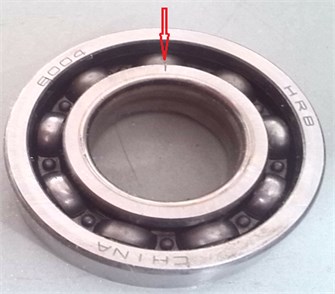
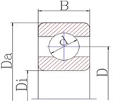
In order to verify the effectiveness of the method, the bearing fault device was designed in this paper. The test-bed is composed of motor, gear box, load, lubrication device, signal acquisition device, a display and so on, as shown in Fig. 1. Bearing model 6004 is chosen, and the crack fault is processed artificially. The test information is shown in Table 1, and the experiment and bearing fault location are shown in Fig. 2.

Table 1The size information of bearing

Name (unit)	Inner ring diameter	Outer ring diameter	Rolling body diameter	Pitch diameter
mm	20	42	6.35	31

Fig. 1The bearing test stand

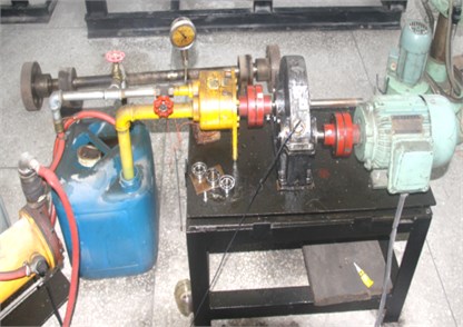
Fig. 2The type of 6004 bearing and fault location

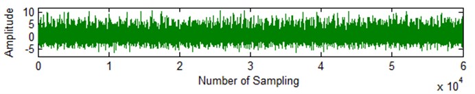
Set the sampling frequency to 10.24 kHz, the speed of the bearing is 2945 r/min. The vibration signal acquired is shown in Fig. 3.

Fig. 3The original signal

According to bearing structure, size and speed, after calculation, the theory failure frequency of bearing inner ring is 266.7 Hz. The frequency of outer ring is 176 Hz, and the rolling element is 115 Hz. According to the theory of Hilbert-Huang, the signal processing is carried out, 16 IMFs and the residual r16 of the signal are obtained.

Table 2The components of the principal component variance energy percentage

Name	Variance	Variance percentage (%)	Name	Variance	Variance percentage (%)
Imf1	0.256427	92.29058	Imf9	2.85E-05	0.01024
Imf2	0.004437	1.59688	Imf10	1.92E-05	0.006912
Imf3	0.005718	2.057968	Imf11	7.75E-06	0.002789
Imf4	0.007385	2.657884	Imf12	5.85E-06	0.002107
Imf5	0.003111	1.119747	Imrer‘f13	3.00E-06	0.001081
Imf6	0.000457	0.164541	Imf14	1.16E-06	0.000419
Imf7	0.000457	0.06823	Imf15	9.77E-07	0.000352
Imf8	0.000457	0.020213	Imf16	1.48E-07	5.34E-05

If each signal was disposed after the subsequent processing, the massive component number will cause tedious calculation and a lot of time will be consumed. In order to reduce them, a variance energy method is introduced, which can analyse the related relationship between the original signal and the decomposed signals. Through calculation each principal component and the percentage of the original signal is shown in Table 2. The decomposed signal with the largest correlation coefficient is analyzed with frequency spectrum which is shown in Fig. 4 and the corresponding three dimensional Hilbert calculation is shown in Fig. 5.

Fig. 4The IMF1 component spectrum diagram

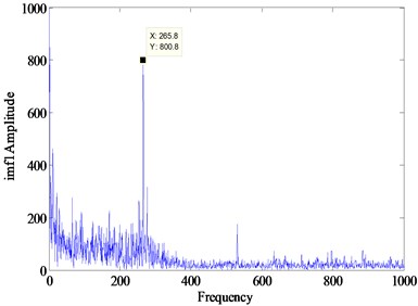
Fig. 5The three dimensional spectrum of signal

As shown above we can see the failure characteristic frequency of the signal is 265.5 Hz, and the corresponding theoretical value is 266.7 Hz, whose nuances is due to the rotation speed fluctuation. So we can diagnose that the bearing fault occurs on inner ring.

Further, the fault law of rolling bearing under different fault levels and load was studied. Due to the limited conditions of the test bench, use the public laboratory bearing test-bed data for vibration signal analysis.

The data provided by the laboratory [11] was collected from a test rig. These bearing fault signals have been widely used to validate the effectiveness of new algorithms for bearing fault diagnosis [12-13]. The experimental setup mainly included a motor (left), a torque transducer and a dynamometer (right). The motor shaft was supported by bearings with the type of 6205-2RS JEM SKF. The bearing inner race, outer race and rolling element were artificially seeded a single point fault by electro-discharge machining respectively. For an inner race localized fault, a rolling element localized fault and an outer race localized fault, the accelerometers were used to sample vibration signals at 12 kHz and installed at 12 o’clock, 3 o’clock and 6 o’clock positions at the drive end respectively.

According to the experiment, choose the size of the bearing parameters shown in Table 3, according to the size of the bearing parameter, the bearing fault frequency is shown in Table 4 through the calculation formula, when the rotating speed is 1797 r/min. The fault is implanted as cylindrical bearing fault artificially, and the fault size in inner raceway is 0, 0.018, 0.036, 0.054 cm, and the load is 0, 1, 2, 3, respectively.

Table 3Bearing size parameters

Name (unit)	Inner ring diameter	Outer ring diameter	Rolling body diameter	Thickness	Pitch diameter
10^-3 m	25.00122	51.99888	7.94004	15.00124	3.90398

Table 4Defect frequencies

Structure	Rotating speed (r/min)	Position	Defect frequencies (Hz)
	1797	Rotate Speed Frequency	29.95
		Ball Pass Frequency Inner Ring	162.2
		Ball Pass Frequency Outer Ring	107.4
		Ball Pass Frequency Cage Train	141.2

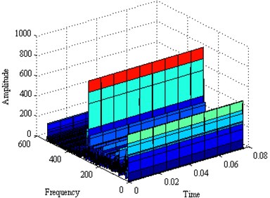
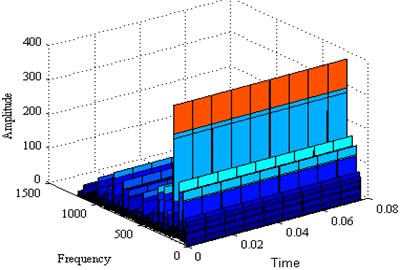
With the same processing method for bearing vibration signal processing research of biggest one signal related component spectrum diagram which is shown in Fig. 7, and the three dimensional spectrum diagram of signal is shown in Fig. 8.

It is clear that the peak value of the signal frequency is 161.7 Hz in the figure, which is near to the theory failure frequency of bearing inner ring 162.2 Hz. The special knot shows that the vibration signal of bearing is inner ring fault signal. At the same time dispose the bearing signals when they are at different load or different fault size, with the same method of signal processing and study the trend research analysis of the bearing amplitude.

Fig. 7IMF1 Component spectrum diagram

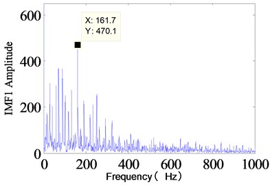
Fig. 8The three dimensional spectrum of signal

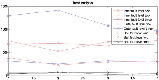
In order to study deeply on the law of bearing fault, different fault grades slots with size of 0.018 cm, 0.036 cm, 0.054 cm are set respectively, keeping the depth constant 0.028 cm and different loads 0, 1 hp, 2 hp, 3 hp are set. The same method, frequency and points are applied in the identical situations. At the same power loaded, it is respectively 0, 1, 2 and 3. The fault level signal processing of the signal spectrum of inner ring is provided in Figs. 9 to 12. The same processing method is used to deal with outer ring and rolling which have the same fault size and load. Red, blue, and black lines represent respectively for inner ring, outer ring and ball signals under the fault level one, two, and three in different load cases.

Fig. 9Fault levels of spectrum diagram with no load

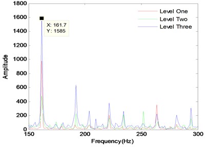
Fig. 10Fault levels of spectrum diagram with load level one

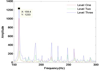
Fig. 11Fault levels of spectrum diagram with load level two

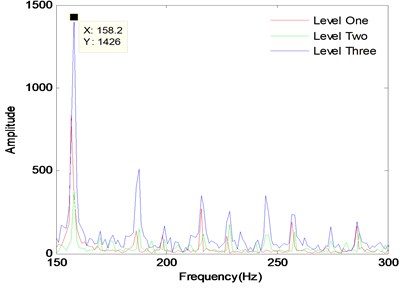
Fig. 12Fault levels of spectrum diagram with load level three

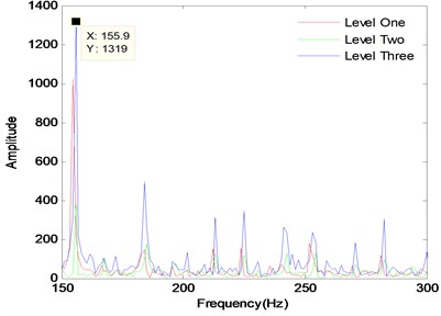
Table 5The detailed spectral analysis results of the fault bearings

Fault Level	Diameter (cm)	Load	Inner ring amplitude	Outer ring amplitude	Ball amplitude
Level One	0.018	0	684.1	1297	41.7
Level Two	0.036	0	385.2	–	66.16
Level Three	0.054	0	749.3	316.3	25.78
Level One	0.018	1	697.6	1413	51.07
Level Two	0.036	1	225.6	–	61.64
Level Three	0.054	1	525.4	253.1	74.22
Level One	0.018	2	642.3	1083	51.23
Level Two	0.036	2	301	–	70.6
Level Three	0.054	2	736.6	320.9	23.32
Level One	0.018	3	911.6	970.8	42.06
Level Two	0.036	3	314.8	–	48.29
Level Three	0.054	3	764.1	307.6	30.82

According to the signal spectrum analysis, it can be clearly diagnosed that the signal fault categories are bearing inner ring. The peak of bearing failure frequency approximate the theoretical value, and the slightly difference happens because of the rotation speed fluctuation. The detailed data analysis is shown in Table 5. For inner ring, under the same load, with increasing size of fault bearing, the frequency amplitude of fault vibration signal is not a gradually increasing trend, as shown in Fig. 13. The changing trend analysis can be seen the failure frequency amplitude of fault level 2 is the smallest, the amplitude of fault level 3 is the biggest, which illustrates that the bearing is under the condition that the vibration amplitude of bearing fault size will appear a smallest point, and then increase with the adding of the fault size. As the load increases, the trend of signal frequency amplitude processing is the same, but the peak value of failure frequency will decrease gradually, which the reason is that as the load is increasing, the speed is reduced, and the theory failure frequency will be reduced as well. For the ball, the trend is almost the same. For the outer ring, fault level one is bigger than fault level three.

Fig. 13The tendency of different fault grades under different loads

4. Conclusions

Based on the designed experimental platform, the HHT was applied to discover the fault law of rolling bearing under different fault levels and loads successfully. The algorithm named variance energy method and correlation coefficients are introduced to solve the problem of EMD decomposition firstly. The different IMF components and the residual one are obtained. Then the fault frequency spectrum and three dimensional Hilbert surface are calculated by our program. Finally, the experimental rolling bearing with different fault levels are designed, and corresponding vibration signals are measured. Results show that with the same fault level, when load is fixed, the failure frequency of the signal can be accurately identified. As the load is increased, the failure frequency is reduced because speed is slow. At the same load, the size of the fault in the process is gradually increasing. Among the four kinds of load spectrum, the frequency amplitude of fault level 2 is straightly minimum, and the frequency amplitude peak value of fault grade is the biggest without intersection. The failure frequency spectrum peak value of bearing vibration signal will not increase with the adding of the fault size, there will be a smallest point and then increase rapidly. In the future study, it should continue to explore high-speed bearing (more than 9000 RPM) diagnosis technology, and study the nonlinear dynamics theory in the diagnosis of the nonlinear dynamic behavior of bearing system, which will provide a beneficial reference for early stage weak fault signal detection.

References

Wang W. J., McFadden P. D. Application of waveletsto gearbox vibration signals for fault detection. Journal of Sound and Vibration, Vol. 192, 1996, p. 927-939.

Search CrossRef
Huang N. E., Shen Z., Long S. R. A new view of non-linear water waves: the Hilbert spectrum. Annual Review of Fluid Mechanics, Vol. 31, 1999, p. 417-457.

Search CrossRef
Montesinos M. E., Munoz-Cobo J. L., Perez C. Hilbert-Huang analysis of BWR neutron detector signals: application to DR calculation and to corrupted signal analysis. Annals of Nuclear Energy, Vol. 30, 2003, p. 715-727.

Search CrossRef
Peng Z., Chu F., Tse P. Detection of the rubbing caused impacts for rotor-stator fault diagnosis using reassigned scalogram. Mechanical Systems and Signal Processing, Vol. 19, 2005, p. 391-409.

Search CrossRef
Hu N. Q., Chen M., Wen X. S. The application of stochastic resonance theory for early detecting rubbing caused impacts fault of rotor system. Mechanical Systems and Signal Processing, Vol. 17, 2003, p. 883-895.

Search CrossRef
Huang N. E., Shen Z., Long S. R. A new view of nonlinear water waves: The Hilbert spectrum. Annual Review of Fluid Mechanics, Vol. 31, 1999, p. 417-457.

Search CrossRef
Norden E. Huang New method for nonlinear and nonstationary time series analysis: Empirical mode decomposition and Hilbert spectral analysis. Proceedings of SPIE, 2000, p. 197-209.

Search CrossRef
Flandrin P., Rilling G., Goncalves P. Empirical mode decomposition as a filter bank. IEEE Signal Processing Letters, Vol. 11, Issue 2, 2004, p. 112-114.

Search CrossRef
Vapnik V. N. Statistical learning theory. Publishing House of Electronics Industry, 2004.

Search CrossRef
Christoph Bandt, Bernd Pompe Permutation entropy: a natural complexity measure for time series. Physical Review Letters, Vol. 88, Issue 17, 2002.

Search CrossRef
CWRU, Bearing Data Center. http://csegroups.case.edu/bearingdatacenter/home.

Search CrossRef
Miao Q., Wang D., Huang H. Z. Identification of characteristic components in frequency domain from signal singularities. Review of Scientific Instruments, Vol. 81, 2010, p. 035113.

Search CrossRef
Miao Q., Cong L., Pecht M. Identification of multiple characteristic components with high accuracy and resolution using the zoom interpolated discrete Fourier transform. Measurement Science and Technology, Vol. 22, 2011, p. 055701.

Search CrossRef

About this article

Received

14 February 2014

Accepted

27 April 2014

Published

30 June 2014

Keywords

rolling bearing

HHT

fault diagnosis

Acknowledgements

Thanks for the support of National Natural Science Foundation of China (No. 51179197), and State Key Laboratory of Ocean Engineering (Shanghai Jiao Tong University) (No. 1009).

This is an open access article distributed under the Creative Commons Attribution License, which permits unrestricted use, distribution, and reproduction in any medium, provided the original work is properly cited.