Abstract
Diagnostics of rotating machines is taking a new step forward with the development of intellectual technologies based on predictive and machine learning tools. Despite having a range of advantages compared to humans in terms of big data processing powers, correlation and various feature extraction possibilities, and swiftness of operation, such systems are limited by measurement system elements in terms of their parameters: sensors and ADCs with their sensitivity properties and accuracy restrictions, microprocessors with limitation of processing powers, etc. Experimental data is used to recreate experimental environment in simulation of induced unbalance. The imitation model is based on rotor dynamics equations of rotor motion, Reynolds equation to estimate reaction forces of a fluid-film bearing and takes into account sensor parameters and position, gear coupling effect and other measurement system elements parameters. The results show that under certain conditions it becomes impossible to successfully track unbalance which in real conditions could lead to malfunction or failure of a rotor machine.
1. Introduction
Importance of successful diagnostics cannot be overestimated in any field of study. Abnormalities of operation are reasonably considered unwanted in any field of study as well. In the field of rotor dynamics this problem has been approached by many researchers and some classic and modern methods could be highlighted. The most used method of fault detection is, of course, signal frequency domain analysis. For instance, in [1] the rotor startup vibrations are utilized to solve the fault identification problem using time frequency techniques. Numerical simulations are performed through finite element analysis of the rotor bearing system with individual and collective combinations of misalignment, rotor cracks and rotor to stator rub. In [2] a very comprehensive study is presented on model-based fault diagnosis in rotor systems with self-sensing piezoelectric actuators. In this research work, the virtual sensor signals are utilized for model-based fault diagnosis in rotor systems, with focus on unbalances in rotors. Unbalance magnitude and phase were estimated in frequency domain using a parameter estimation method by least squares optimization. Novelty of this work is in application of self-sensing piezo-electric actuators in a closed-loop to solve both diagnostics and control tasks. In [3] combined rotor fault diagnosis in rotating machinery using empirical mode decomposition is presented with focus on the main fault modes: unbalance, misalignment, partial rub, looseness and bent rotor. In [4] authors present another interesting case of mode decomposition to identify multi-fault in rotor-bearing system using spectral kurtosis and ensemble EMD. In [5] Identification and diagnosis of concurrent faults in rotor-bearing system is performed using wavelet packet transform and zero space classifiers. While these already classic approaches suit their goal very well in most cases, there is another field of study to take diagnostics on a new level – machine learning and artificial neural networks [6-9].
The present paper intends to look at the problem of fault detection from a different perspective and presents an approach to estimation of what is called ‘detectability’ of a fault mode – evaluation of possibility of detection of a fault based on measurement system parameters with focus on rotor unbalance.
2. Experimental setup and results
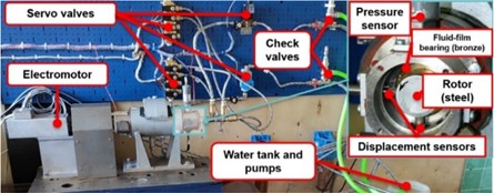
In Fig. 1 the overview of the test rig is presented. The rotor system consists of a hollow rotor with diameter of 40 mm in the thickest sections where bearings are located and 39.8 mm elsewhere. Mean wall thickness is about 1.6 mm but varies slightly along the rotor. It is made of steel and with 3D printed auxiliary components – gear coupling and rear cap - weighs around 0.6 kg. Close to the rear end of the rotor a hybrid fluid-film bearing is installed, lubricant – water – is supplied axially so that the bearing is fully lubricated but pressure doesn’t exceed ambient level and the bearing does not operate in hydrostatic regime. Perpendicular to each other two displacement sensors AE051.05.07 with matching devices D210A-C.05.05 are mounted in the bearing housing. Data from these sensors is acquired using National Instruments NI cDAQ chasse module and analog input module NI 9205. The electromotor rotates at a constant speed of about 2700 rpm. The setup along with some results on various fault modes focusing on aerated lubricants is presented in more detail in [10].
In Table 1 main parameters of the test rig elements are presented. The same parameters are used for modeling below.
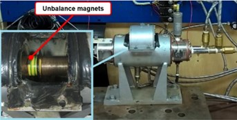
Fig. 1a) Test rig, b) opened hatch to mount unbalance magnets
a)
b)
Table 1Main parameters of the test rig
Element | Parameter | Value (range) |
Electromotor | Rotation frequency | ~ 45 Hz |
Rotor | Diameter | 40 mm |
Length with coupling | 397 mm | |
Mass | ~0.6 kg | |
Bearing | Distance to the coupling | 352 mm |
Radial clearance | 75·10−6 m | |
Length | 0.02 m | |
Lubricant | Dynamic viscosity | 1·10−3 Pa·s |
Displacement sensors | Output signal | 0..10 V |
Measurement range | 0.1..2.1 mm | |
Accuracy | ~1·10−6 m | |
Recovery time | ~5 ms | |
ADC | Bit depth | 16 bit |
Sampling frequency | 1 kHz |
In order to estimate the influence of the induced unbalance on the position measurements a series of test was carried out with two magnets attached to the rotor about 4 g each. They were mounted in the middle of the rotor length on top of each other (see Fig. 1(b)) on a layer of duct tape in order to be able to be removed easily.
3. Imitation model of the test rig
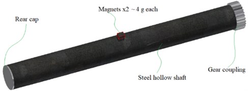
In Fig. 2 a schematic of the rotor-bearing system is presented. Rotor weight is distributed between the coupling and the bearing, and the latter bears a very light load which results in very low eccentricity. The rotor has four degrees of freedom and is modelled assuming that it has no thickness variation using Autodesk Inventor software to determine coordinates of the center of mass, polar and diametral moments of inertia and unbalance. PLA/ABS plastic was used for material settings for the rear cap and the gear coupling, steel was used to model the rotor. Overview of the model of the unbalanced rotor with magnets is presented in Fig. 3. Gear coupling is modelled as constant stiffness and damping.
Fig. 2Calculation schematic for the rotor dynamics
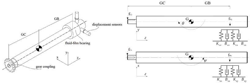
Fig. 33D model of the hollow rotor with unbalance magnets
Forces and that act on the bearing are counteracted by reaction forces of the fluid film in the equilibrium position so that sum of all forces is equal to zero. Displacement from this position cause additional forces to occur that are non-linear in reality, however, can be linearized around the fixed point being the equilibrium position given that displacements are infinitesimal. This is very well-known and widely used procedure [11].
In order to find the equilibrium position equations of hydrodynamic lubrication theory must be solved to determined pressure distribution within the fluid film. Integration of pressure distribution allows determination of force components of the fluid-film reaction force [12]. Geometric parameters in Fig. 5 and Table 1 and linearization technique allows the following equations of rotor motion to be obtained [13]:
where is rotor mass, , and are forces carried by the coupling, the bearing and induced by unbalance respectively, and are distances to the coupling and to the bearing respectively, and are polar and diametral moments of inertia and , , and are respective coordinates. Force components generated in the bearing are as follows:
where and are stiffness and damping coefficients along respective axes. Finally, forces due to unbalance are as follows:
where is unbalance, is angular velocity and is phase shift. For real cases most of the time the exact values of unbalance are rarely known, instead some ranges could be specified. However, in the present case no information on unbalance is given beforehand, so the values of are going to be determined using experimental data.
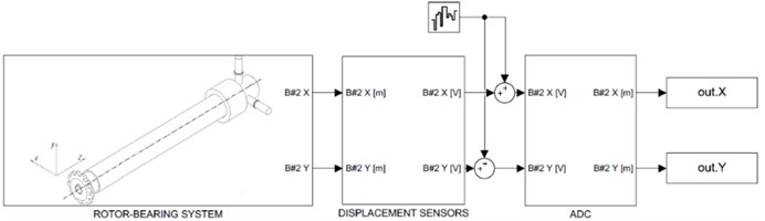
Modeling of additional elements was done in Simulink. Operation of displacement sensors was simulated using the following transfer function:
where is sensor gain and is time constant based on recovery time from Table 1. ADC was modelled using datasheet data on accuracy, and sampling time and bit depth from Table 1. Before signals enter the ADC they are exposed to white noise with power to match experimental data. Operation of the ADC was modelled with First-Order Hold and Quantization blocks in Simulink. In Fig. 5 the Simulink imitation model is presented.
In the imitation model the “Rotor-Bearing System” block numerically solves Eqs. (1-3), the “Displacement Sensors” block is Eq. (4).
Fig. 5Simulink imitation model
4. Results and discussion
Ten experimental datasets of normal operation and ten datasets with induced unbalance were analyzed in frequency domain to determine average parameters of the rotor orbit. The results are shown in Table 2.
It could be seen, that additional unbalance results in about two times bigger amplitudes with amplitudes remaining essentially the same. In order to model similar behavior the rotor model was used as described above given the inertia parameters obtained from the Inventor model (Table 3).
It has to be noted that the ‘normal’ case rotor model has zero unbalance because all of its parts are symmetric, but since in reality this is hardly possible, experimental data from the ‘normal’ set of tests was used to have some initial unbalance. Trial and error allowed estimation of initial unbalance to be about 1 mm with zero phase, with having 29 % error of the simulated magnitude along and 8 % error of that along compared to mean values in Table 2. Such big error along is presumably connected with radial gap shape deviation from ideal, it was determined later that radial gap in direction was less than that along by 25 µm. Compared to one of the ‘normal’ experimental cases, results of simulation of the ‘normal’ case are presented in Fig. 6.
Table 2Experimental results processing
Case | Mean magnitude , µm | Mean magnitude , µm | Mean frequency, Hz |
Normal | 13.5 | 9.5 | 45.8 |
Unbalance | 13.3 | 20.1 | 45.7 |
Table 3Inertia parameters of the modelled rotor
Case | Polar moment, , kg·m2 | Diametral moment, , kg·m2 | Mass, kg | Coordinates of , mm |
Normal | 2.03×10⁻⁴ | 6.73×10⁻³ | 0.552 | (0, 0, 189) |
Unbalance | 2.08×10⁻⁴ | 6.74×10⁻³ () 6.73×10⁻³ () | 0.559 | (0.005, 0.327, 189) |
Fig. 6“Normal” case simulation
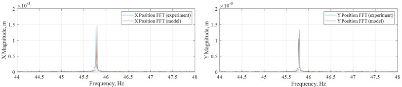
Fig. 7“Unbalance” case simulation
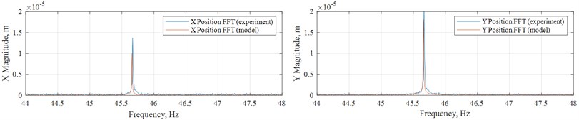
The imitation model in Fig. 5 along with the rotor model with induced unbalance in Fig. 4 were used to recreate the ‘unbalance’ case. It could be seen that the center of mass are no longer on the axis, and this results in additional 0.327 mm. Added to the determined initial unbalance of approximately 1 mm with zero phase, this time due to changed center of mass coordinates phase changes to 0.0153 rad. This geometrically results in 1.32 mm. In this case modelling of such case using inertia parameters from the corresponding case in Table 3 yields 32 % error of the simulated magnitude along and 11 % error of that along compared to mean values in Table 2. Adjusting of unbalance and phase within geometric restrictions via trial and error slightly improved the results to 26 % error of the simulated magnitude along and 13 % error of that along with 1.3 mm and 0.0768 rad. Compared to one of the ‘unbalance’ experimental cases, results of simulation of the ‘unbalance’ case are presented in Fig. 7.
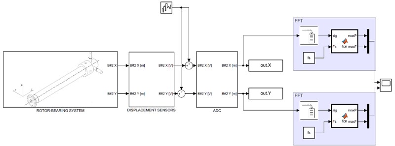
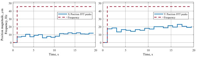
The results shown above allow use of the developed model to study the influence of various parameters of the measurement system on the possibility to detect the change of unbalance during operation. The model was augmented with online FFT blocks that acquire 1024 buffered samples and plot peak magnitudes along each coordinate and corresponding frequency (Fig. 8). Should magnitude change this must be able to be noticed from this data, so the following analysis is focused on sensitivity of quality of these measurement to sensor and ADC parameter. A sample of what measurement data looks like when it reaches the monitoring and diagnostics system is presented in Fig. 9. In simulation unbalance changed from the “normal” case to the “unbalance” case when simulation time reached 10 s.
Fig. 8Augmented model for online FFT analysis
A series of numerical tests were carried out to determine sensitivity of the measurement system, and it has been determined that the most influential parameters of the system were: displacement sensors accuracy (the biggest effect), noise power (the second biggest effect), ADC bit depth (the third highest), other parameters had more or less the same impact: sampling frequency, buffer size. It shall be noted, of course, that the main parameter that influenced this estimation was indeed unbalance.
The present paper investigated imitation modeling of fault mode in a rotor system, its analysis in the frequency domain and simulation of monitoring and diagnostics system in order to determine which of its parameters influence its performance the most. Future work is going to be focused on derivation of an analytical parameter that could allow determination of detectability of a fault in a rotor system given main measurement system parameters.
Fig. 9Operation of the monitoring and diagnostics system
References
-
Harish Chandra N., SekharA. S. Fault detection in rotor bearing systems using time frequency techniques. Mechanical Systems and Signal Processing, Vol. 72–73, 2016, p. 105-133.
-
Sankaranarayanan R. A. Model-Based Fault Diagnosis in Rotor Systems with Self-Sensing Piezoelectric Actuators. Ph.D. Thesis, Darmstadt Technical University, 2017, p. 151.
-
Singh S., Kumar N. Combined rotor fault diagnosis in rotating machinery using empirical mode decomposition. Journal of Mechanical Science and Technology, Vol. 28, 2014, p. 4869-4876.
-
Gong X., et al. Identification of multi-fault in rotor-bearing system using spectral kurtosis and EEMD. Journal of Vibroengineering, Vol. 19, Issue 7, 2017, p. 5036-5046.
-
Jiang F., et. al Identification and diagnosis of concurrent faults in rotor-bearing system with WPT and zero space classifiers. Journal of Vibroengineering, Vol. 16, Issue 2, 2014, p. 901-912.
-
Zhao R., et al. Machine health monitoring using local feature-based gated recurrent unit networks. IEEE Transactions on Industrial Electronics, Vol. 65, Issue 2, 2018, p. 1539-1548.
-
Liu R., et al. Artificial intelligence for fault diagnosis of rotating machinery: a review. Mechanical Systems and Signal Processing, Vol. 108, 2018, p. 33-47.
-
Saidi L., et al. Wind turbine high-speed shaft bearings health prognosis through a spectral kurtosis-derived indices and SVR. Applied Acoustics, Vol. 120, 2017, p. 1-8.
-
Diez Olivan A., et al. Data fusion and machine learning for industrial prognosis: trends and perspectives towards Industry 4.0. Information Fusion, Vol. 50, 2019, p. 92-111.
-
Kornaeva E. P., et al. Application of artificial neural networks to diagnostics of fluid-film bearing lubrication. IOP Conference Series Materials Science and Engineering, Vol. 734, 2020, p. 9.
-
Savin L. Solomin O. Modeling of rotor systems with support of liquid friction: monograph. Mechanical Engineering – 1, 2006, p. 444, (in Russian).
-
Hori Y. Hydrodynamic Lubrication. Springer-Verlag, Tokyo, 2006, p. 238.
-
Friswell M. I., et al. Dynamics of Rotating Machines. Cambridge University Press, 2015, p. 650.
Cited by
About this article

The work has been carried out within the Project No. 05.607.21.0303 “Development of an Intelligent Monitoring Technology and a Prototype of the Hardware and Software Complex for Safety of Energy Complex Facilities” supported by the Federal Target Program “Research and Development in Priority Areas for the Development of the Scientific and Technological Complex of Russia for 2014-2020” by the Ministry of Science and Higher Education of Russian Federation (unique identifier of the research RFMEFI60719X0303).
Authors would also like to thank Alexey Kornaev and his team for the experimental data they kindly provided for our simulation.
