Abstract
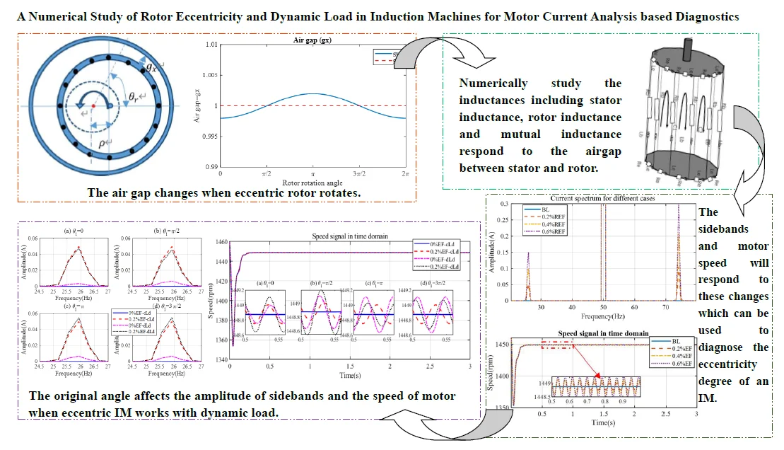
The asymmetry in the manufacturing and assembling is the common issue of rotor systems. Different degrees of errors are inevitable in alternating current (AC) motors, which causes degraded performances. Furthermore, around 80 % of mechanical faults link to rotor eccentricity. The eccentricity faults (EFs) generate excessive mechanical stress and then lead to fatigue in the other parts of the motor. Motor current signal analysis (MCSA) can be used to diagnose induction machine (IM) faults. As the EF leads to an unequal air gap when the rotor rotates, the inductance of IM also responds to the EF. Moreover, the dynamic load is a typical situation due to residual dynamic unbalance and misalignment. To study how EFs and dynamic load affect the stator current. The current model of symmetrical motor, asymmetrical motors with three-level EFs and with dynamic load are investigated numerically. The correctness of models is verified through experimental study. The results show the level of EF affects the sideband peak values significantly in the stator current spectrum. These findings will provide a foundation for the accurate diagnosis of motor health conditions.
Highlights
- The inductances change when eccentric degree changes.
- Motor speed fluctuates and sidebands amplitude increase as the eccentricity increases.
- The original angle affects sidebands and speed when eccentric IM works with dynamic load.
1. Introduction
Eccentricity faults (EFs) refer to the air-gap space between stator and rotor that varies when the induction machine (IM) is working [1]. 80 % of mechanical faults result in rotor eccentricity [2]. The eccentric motor generates excessive mechanical stress and then leads to fatigue in the bearing [3]. Although motor manufacturers make every effort to minimise the asymmetry in the manufacturing and assembling, the error still exists [4]. As Fig. 1 shows, eccentricity faults include static eccentricity (SE) fault, dynamic eccentricity (DE) fault and mixed eccentricity fault of SE and DE [5]. SE refers to the air-gap space is fixed when the rotor rotates. However, the air gap at different radians is unequal as Fig. 1(b) shows. As illustrated in Fig. 1(c), DE fault refers to the space change periodically at a fixed circumferential position periodically. Fig. 1(d) shows the mixed eccentricity of SE and DE.
Misalignment is the main cause for SE [1]. Misalignment causes the rotor’s physical centre away from the stator centre. DE usually results from oval cores, bent shaft and worn bearings [6].
Motor current signal analysis (MCSA) is an effective method used to diagnose EF faults [7], [8], [9]. To study how EFs affect the stator current. The current model of symmetrical motor, asymmetrical motors with three-level EFs are investigated numerically.
Rotor eccentricity results in an unbalanced magnetic pull. Consequently, vibration, acoustic noise, increasing in stator-rotor rub, bearing wearing and/or rotor deflection failure will happen. It also, which might have bad effects on the stator or rotor core, conductor, and/or insulation [10]. The low-frequency range of dynamic eccentricity frequency is:
The fault related sidebands around the supply frequency are:
where and represent supply frequency and rotating frequency, respectively. 1, 2, 3… represents the order of the sideband.
Dynamic load faults come from external faults instead of from an IM. It is mainly caused by gearbox transmission failure, load imbalance and misalignment [11]. The load faults primarily cause a non-constant load torque with time [12].
If the load torque oscillates as the IM working, the current will be modulated with spectral components related to abnormal load faults [13]. The supply current signal in the healthy motor is sinusoidal. Any torque oscillation at a multiple of the rotational speed will produce stator currents at eccentricity frequency (Eq. (1) (2)) [14].
The rest of this article consists of four sections. Section 2 proposes a motor current model of symmetrical motor and asymmetrical motor with different level EFs. Section 3 carries out simulation analysis using MATLAB software. Section 4 set up the experiment and presents the test procedure to verify the proposed model. Section 5 analyses the test data and discuss the results. Section 6 concludes this work.
Fig. 1Different types of air-gap eccentricity faults
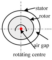
a) Healthy case
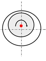
b) Static eccentricity
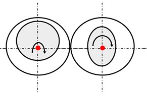
c) Dynamic eccentricity
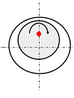
d) Mix eccentricity
2. Motor current models
2.1. Motor current model of healthy motor
A three-phase IM has three-phase distributed windings, displaced relative to each other by 120 degrees, each of the stator and rotor winding circuits has the same form of the voltage equations. According to Kirchhoffs Voltage Law the voltage equation can be given as [15]:
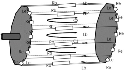
where and are the voltage and current vector matrices, respectively, represents the motor resistance and is the inductance matrix. An equivalent circuit of the symmetrical rotor is shown in Fig. 2. If is the voltage vector, then:
where and represent stator voltage vector and rotor voltage vector, respectively. , , are the voltage of phases A, B, and C. There are bars in the rotor. represent the voltage of the th rotor bar. is the voltage in the end ring. If is the current vector, then:
where and represent stator current vector and rotor current vector, respectively. , , are currents of phases A, B, and C. represents the current of the th rotor bar. is the current in the end ring.
Fig. 2Equivalent circuit of the asymmetrical rotor
The inductance is expressed as:
where is the stator self-inductance, is the stator-to-rotor inductance, is the rotor-to stator inductance, and is the rotor self-inductance. see Eqs. (7) to (20):
The inductances are given as follows:
where: – permeability of free space, – effective radius of the air gap, – machine stack length, – the winding functions for windings and respectively which depends solely on the spatial stator circumferential position , – air gap function, – rotor circumferential position.
2.1.1. Stator self-inductance calculation
According to the matrix equations, the stator-to-stator inductance can be derived as [16]:
where:
where is constant and represent the airgap for the healthy motor. represents pole pairs of induction machines.
is the number of the stator turns similarly:
where .
2.1.2. Stator-to-rotor inductance calculation
Similarly:
2.1.3. Rotor self-inductance calculation
where the (, 1, 2, 3,…, ) can be calculated using Eq. (20):
is the resistance matrix [8] and is given in Eq. (21). The matrices of stator resistance and rotor resistance are given in Eqs. (22) and (24), respectively:
According to Eq. (3), the current differential equation of the healthy motor is derived as follows:
To obtain the speed and displacement of the rotor which are required to calculate the cross inductances in Eqs. (13)-(18), dynamic load balance equation is given as follows:
where represents mechanical inertial. represent external load. The electric torque is given in Eq. (27) [15]:
2.2. Motor current model of eccentricity motor
According to the current differential equation of the healthy motor in Eq. (25), the current will respond to the changes in the voltage , inductance , resistance and rotor angular speed . For the asymmetrical motor, the voltage , resistance R and angular speed are the same as for a healthy motor.
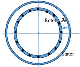
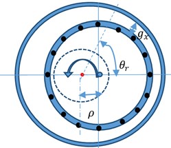
According to Eq. (8), The inductance is affected by the air-gap . For a healthy motor, the air gap () is constant, see Fig. 3(a). With an eccentricity fault, the air-gap at a given point on the stator between the stator and rotor will change () as the rotor rotates, see Fig. 3(b). Therefore, the inductance matrix for a motor with an eccentricity fault () will be different from that of a healthy motor ().
The air-gap distance for an eccentric rotor is:
where is degree of eccentricity.
Fig. 3Eccentricity fault: schematic diagram
a) Healthy motor
b) Motor with eccentricity fault
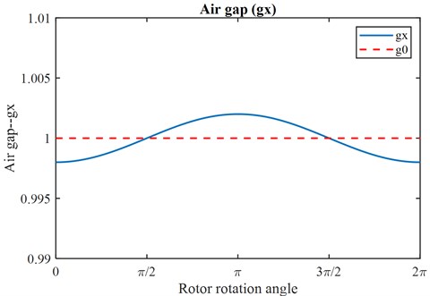
For 1, and 0.001 as an example, the air gap changes with the rotation angle, as shown in Fig. 4.
Fig. 4Schematic diagram of change in the air gap, where gx=1(1-0.001cosθr)
The inductance of the eccentric motor is given in Eq. (29):
The air gap changes as the rotor rotates, the stator self-inductance (), rotor self-inductance () and mutual inductance of an eccentric motor () are given as follows:
Therefore, the current differential equation for the motor with an eccentricity fault can be written as:
2.3. Motor current model of dynamic load
When there are time-varying external loads such as rotor DE and unbalances, the airgap, inductance, and resistance are the same as the healthy condition. The variable parameters would be the external load which can be modelled by Eq. (34):
where is constant load. is the coefficient of the dynamic load, represent the original angle. The external load can be set as a constant or time-varying one to correspond to different load scenarios according to set the coefficient .
Combining the resistance and inductance matrices with the current differential equation, etc., the current of the healthy motor, the motor with different degree eccentricity and motor with dynamic working load can be calculated and simulated as described in Section 3.
3. Eccentricity motor simulation analysis
3.1. Motor current characteristics with eccentricity
The parameters of the simulation at set up are as shown in Table 1.
Table 1Parameters used in simulations
Category | Main parameters | Technical data |
Motor | Supply power | 3.0 kW |
Supply voltage () | 220 V | |
Supply frequency () | 50 Hz | |
Torque () Mechanical inertia () | 15.7 N·m 0.089 | |
Angular speed () | 152.89 rad/s | |
Rated speed | 1460 rpm | |
Number of bars () | 28 | |
Number of turns per stator phase | 183 | |
Pole pairs () | 2 | |
Phase | 3 | |
Resistance | Stator resistance ) | 4.4 Ω |
Rotor bar resistance () | 3.8×10⁻⁵ Ω | |
End ring resistance () | 4.75×10⁻⁵ Ω | |
Inductance | Permeability of free space () | 1.26×10⁻⁶H/m |
Effective radius of the air gap () | 0.0455 m | |
Machine stack length () | 0.125 m | |
Others | Sampling frequency | 2000 Hz |
Sampling time | 3 s |
Based on the theoretical study in Section 2 and the parameter setting above, a simulation was carried out by solving the differential equations Eq. (24) and (32) using solver ode45 in MATLAB (Version: 2020a) software. The stator current of the healthy motor is shown in Fig. 5. The stator current is a sine wave, see Fig. 5(a). The current spectrum in Fig. 5(b) shows a substantial peak at the supply frequency is 50 Hz, this will be the case in all the following simulations of the rotor and stator current spectrums.
For eccentricity studies, the simulation was implemented using the same parameters defined for the healthy model, but Eq. (29) (30) (31) are set with different degrees of eccentricity degree () as shown in Table 2.
Fig. 5Stator current signal for the healthy motor
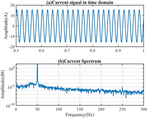
Table 2Parameters used for simulating different degrees of eccentricity
Motor health condition | Degree of eccentricity () | Value | Notation in Figures | Others |
Healthy motor | 1 | 0 % | BL | Comparison case |
Motor with eccentricity fault | 2 | 0.2 % | 0.2 % EF | Study cases |
3 | 0.4 % | 0.4 % EF | ||
4 | 0.6 % | 0.6 % EF |
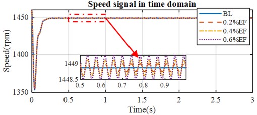
According to the analysis made in Section 1, the eccentricity frequency occurs at frequencies of . The supply frequency, is 50 Hz. the rotational frequency, is calculated from the rotational speed. and the eccentricity fault 50±24.1 ≈ 25.9 and 74.1 Hz. The simulated stator current spectrum in Fig. 7 shows sidebands around the 50 Hz peak at fault frequencies of 25.9 Hz and 74.1 Hz for study cases but no sidebands for the healthy cases (BL). Furthermore, when an eccentricity was introduced, the speed fluctuated, see Fig. 6. The speed fluctuation increased with the degree of the eccentricity as did the amplitude of the sidebands.
Fig. 6The simulated speed with eccentricity faults
3.2. Influences of dynamic load on motor current characteristics with eccentricity
To simulate dynamic loads, the torque balance equation of Eq. (27) is set up as constant and dynamic as follows.
Fig. 7Simulated stator current spectrum with eccentricity faults
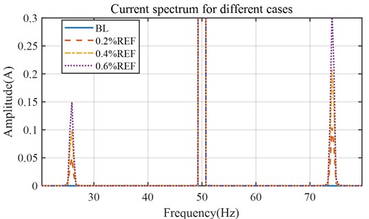
Table 3Parameters used for simulating dynamic load
Cases | Coefficient of the dynamic load () | Degree of eccentricity () | Notation in Figures | Original angel |
Constant load | 0 | 0 % | 0 % EF-cLd | 0; ; ; |
0.2 % | 0.2 % EF-cLd | |||
Dynamic load | 0.02 | 0 % | 0 % EF-dLd | |
0.2 % | 0.2 % EF-dLd |
To better understand how the original angle affects the diagnosis results. All the cases with for original angles ( 0; ;;) respectively.
Fig. 8 shows the speed of the healthy case (0%EF-cLd) is stable but with eccentricity or dynamic load fluctuation. When the motor with a 0.2 % eccentricity, the speed under dynamic load fluctuates more than under constant load. Fig. 8 illustrate the speed of different cases with the original angles () of 0, ,,. Fig. 8(a) and 8(b) show when and , under the same dynamic load, the speed fluctuates more when eccentricity getting severe. However, the Fig. 8 (c) and (d) show when and , under the same dynamic load, the speed fluctuates less when eccentricity getting severe.
Fig. 8The simulated speed with different degrees of eccentricity and dynamic load
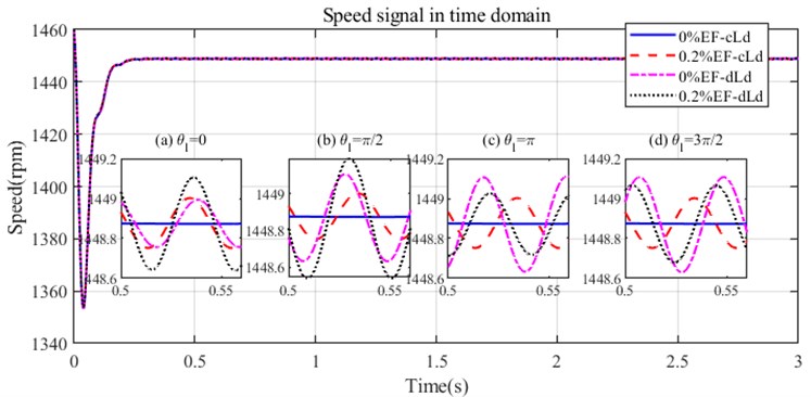
Fig. 9Simulated current spectrum with eccentricity and dynamic load (θl=0)
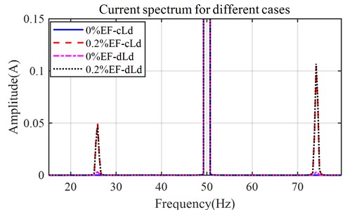
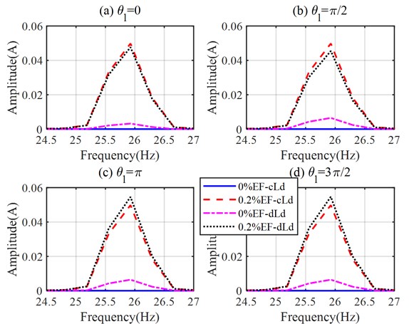
Fig. 9 shows the current spectrum of different dynamic load cases when . there are sidebands for eccentricity or dynamic load cases. Take the lower sideband as the example, to better compare the sideband amplitude when changes, Fig. 10 illustrate the current spectrum of different cases with the original angels () of 0, ,,. For a balance (no eccentricity) motor, the sidebands of cases under the dynamic load are higher than that under constant load. However, when the motor is with eccentricity, the sidebands of the dynamic load cases in the spectrum a related to the original angle.
Fig. 10Left sideband for different original angle a) θl=0, b) θl=π2, c) θl=π, and d) θl=π2
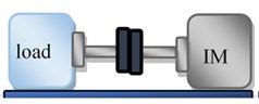
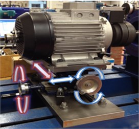
4. Experimental setup and test procedure
An IM test rig (Fig. 11) is set up to validate the proposed simulation. It includes an induction motor and a generator, which is mechanically coupled with the motor to provide different loads. Three induction motors with the same specifications but different health conditions are tested subsequently. The specifications of the motor are listed in Table 4.
To verify the efficiency of the proposed method under different operations. In the experiment, all the cases are tested under five representative loads (0 %, 20 %, 40 %, 60 % and 80 %) at 100 % rated speed. All the operating conditions are summarized in Table 5. The eccentricity level of healthy case <= 0.07 mm, of the eccentric motor are 0.5 mm and 1 mm respectively as shown in Fig. 12. Note that the motors are controlled under openloop mode, a no feedback mechanism that keeps a constant main supply frequency 50 Hz at 100 % rated speed.
Fig. 11The IM test rig
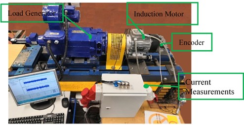
Fig. 12Schematic diagram showing the degree of misalignment

a) Baseline (<= 0.07 mm)
b) Misalignment 1 (0.5 mm)

c) Misalignment 2 (1 mm)
Table 4Specification of test motor
Parameters | Value |
Rated voltage (/) | 230/400 V |
Rated current (/) | 15.9/9.2 A |
Motor power | 4 kW |
Number of phases | 3 |
Pole Pairs | 2 Pairs |
Supply frequency | 50 Hz |
Rated speed | 1420 rpm |
Number of rotor bars | 28 |
Table 5Test operations for EF test
Degree of misalignment (mm) | Load (%) | Speed (%) | ||||
<= 0.07 | 0 | 20 | 40 | 60 | 80 | 100 |
0.50 | 0 | 20 | 40 | 60 | 80 | 100 |
1.00 | 0 | 20 | 40 | 60 | 80 | 100 |
Fig. 13a) Eccentricity measurement and, b) introducing the eccentricity into the induction motor
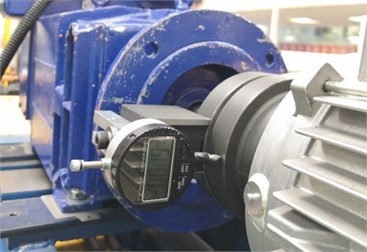
a) Eccentricity measurement
b) Introducing eccentricity
The eccentricity fault was seeded into the test rig with different severities. As mentioned in Section 1, misalignment is the main cause of static EF. Therefore, misalignment is made in this research experimental study to make EF. The degree of eccentricity was measured using a dial indicator. The dial indicator was installed on its magnetic base, which can be attached to the coupling to guide the positioning of the motor, see Fig. 13(a). Fig. 13(b) illustrates changing the eccentricity by adjusting the two-axis compound table. The parameters of the instrument are listed in Table 6.
Table 6Parameters of dial indicator
Manufacturer | Matrix coventry gauge and tool |
Range | 0-12.7 mm / 0.5 inch |
Resolution | 0.001 mm / 0.00005 inch |
5. Data analysis and result discussion
The supply frequency, in openloop control mode is constant at 50 Hz. The rotational frequency, , can be calculated using the encoder signal. According to Eq. (1), the eccentricity frequency, equals the rotational frequency The fault information will be contained in the modulation of the supply signal (50 Hz). Take the lower sideband () frequencies of the two EF cases as the example. According to Eq. (2), the lower eccentricity-related sideband frequency equals the supply frequency minus the eccentricity frequency ( = ) and they are listed in Table 7.
Table 7Eccentricity frequency for healthy motor and EF cases
Case | Eccentricity frequency (Hz) | ||||
Load: 0 % | 20 % | 40 % | 60 % | 80 % | |
Healthy | 24.95 | 24.77 | 24.57 | 24.32 | 24.03 |
EF0.5mm | 24.95 | 24.77 | 24.55 | 24.30 | 24.02 |
EF1mm | 24.95 | 24.77 | 24.55 | 24.32 | 24.02 |
Table 8Frequency of lower sideband for healthy motor and EF cases
Case | Sideband frequency (Hz) | ||||
Load: 0 % | 20 % | 40 % | 60 % | 80 % | |
Healthy | 25.05 | 25.23 | 25.43 | 25.68 | 25.97 |
EF0.5mm | 25.05 | 25.23 | 25.45 | 25.70 | 25.98 |
EF1mm | 25.05 | 25.23 | 25.45 | 25.68 | 25.98 |
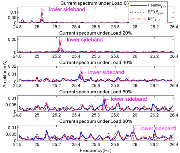
The current spectrums of healthy motor (HealthyOP, where the subscript OP stands for openloop control mode), motor with 0.5 mm eccentricity (EF0.5OP) and motor with 1 mm eccentricity (EF1OP) is shown in Fig. 14. The supply frequency is stable at 50 Hz under all three conditions. According to the lower EF sidebands in Table 8, the sidebands around 25 Hz are related to an EF. Under 0 % load (solid dark blue line in Fig 14), the amplitude of the sidebands increases as the eccentricity increases. However, the sidebands under other loads are not clear. To better observe the sideband amplitude, the lower sidebands under the three operating conditions in the range from 25 Hz to 26 Hz are shown in Fig 15.
Fig. 15 shows the frequencies of the EF sidebands increase as load increases. Unlike the BRB fault, the amplitude of the fault indicator for the EF decreases as the load increases. The fault indicators are clear to observe under light loads, but almost buried in the noise under heavy loads, especially 60 % and 80 % loads.
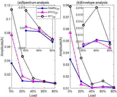
Using the Hilbert-based envelope method to extract the fault information, the derived spectrum in Fig. 16 confirms that envelope analysis can extract eccentricity information from the current signal. Similarly, with the spectrum analysis, the peak amplitudes at fault frequencies in the envelope spectrum decrease as the load increases and are nearly buried in the noise and interference under high loads, at and above 40 %, 60 % and 80 %, see Fig. 17(b). Compared with spectrum analysis (Fig. 17(a)) envelope analysis shows better performance in separating the EF1OP case with the highest amplitudes at 0 % to 60 % loads but shows better capability when separating healthy and EF0.5OP under 20 %, 60 % and 80 % loads.
Fig. 14Current spectrum of a) healthy motor, b) motor with 0.5 mm EF, c) motor with 1 mm EF for various loads
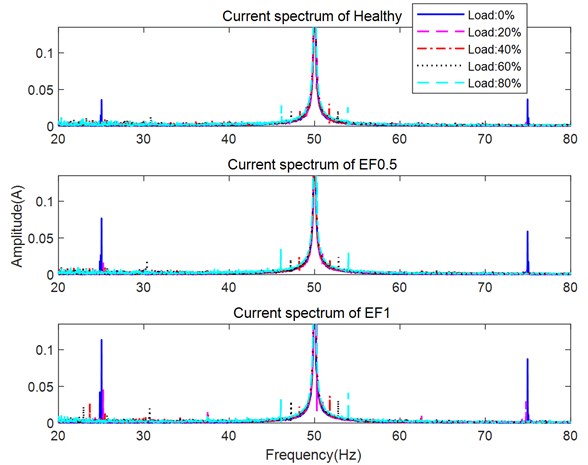
Fig. 15Current spectrum showing lower sideband for healthy motor and motor with EF0.5OP, and motor with EF1OP under various loads
The amplitudes of the lower sidebands in the spectrum, see Fig. 17(a), increase as the degree of eccentricity increases under loads of 0 %, 20 %, 40 %, and 60 %. But it is difficult to separate the two eccentricity levels with a load of 80 %.
The analysis results under different loads show the fault indicator increase when the eccentricity increase which consistent with the proposed model analysis under different loads, especially under light loads, which verify the correctness of the model of eccentricity. The result under higher loads does perform as well as under light loads which illustrate the eccentricity motor is more difficult to diagnose under heavier loads.
Fig. 16Envelope spectrum for healthy motor and motor with EF0.5OP, and motor with EF1OP under various loads
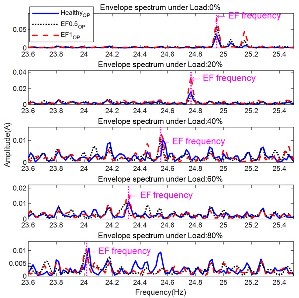
Fig. 17Amplitudes of EF indicators under various loads using a) spectrum analysis b) envelope analysis
6. Conclusions
This study develops AC motor models with eccentric effects. It firstly studies motor current spectrum behavior when there are different degrees of rotor eccentricity along. Subsequently, the behavior is also investigated when dynamic loads were applied to the eccentric motor, which is a typical situation due to residual dynamic unbalance and misalignment. The key findings of this study can be summarized as follows: the eccentricity fault leads to changes in air-gap flux as the rotor rotates. The inductance, including the stator self-inductance, rotor self-inductance and mutual inductance will change with the air gap. The simulated stator current spectrums for different degrees of eccentricity fault and dynamic load fault show that in the baseline case (healthy motor) no fluctuation occurred in the motor speed and no sidebands are observed. However, introducing an eccentricity fault causes fluctuation in the motor speed, which increases as the eccentricity fault increases. Eccentricity induces fault-related sidebands, which increases in amplitude as the eccentricity fault becomes more serious. For the balance (no eccentricity) motor, the sidebands of cases under the dynamic load are higher than under constant load. And the speed fluctuates more than the constant load cases. However, when the motor is with eccentricity, the sidebands of the dynamic load cases in the spectrum and the speed fluctuations related to the original angle. Among them, the amplitude at a rotating frequency which regarded as the fault indicator has been experimentally certificated increase when eccentricity getting serious.
References
-
Y. Liu and A. M. Bazzi, “A review and comparison of fault detection and diagnosis methods for squirrel-cage induction motors: State of the art,” ISA Transactions, Vol. 70, pp. 400–409, Sep. 2017, https://doi.org/10.1016/j.isatra.2017.06.001
-
P. C. Sen, Principles of Electric Machines and Power Electronics. John Wiley & Sons, 2007.
-
S. Chapman, Electric Machinery Fundamentals. Tata McGraw-Hill Education, 2005.
-
W. T. Thomson and A. Barbour, “On-line current monitoring and application of a finite element method to predict the level of static airgap eccentricity in three-phase induction motors,” IEEE Transactions on Energy Conversion, Vol. 13, No. 4, pp. 347–357, 1998, https://doi.org/10.1109/60.736320
-
D. Hyun, S. Lee, J. Hong, S. Bin Lee, and S. Nandi, “Detection of airgap eccentricity for induction motors using the single-phase rotation test,” IEEE Transactions on Energy Conversion, Vol. 27, No. 3, pp. 689–696, Sep. 2012, https://doi.org/10.1109/tec.2012.2198218
-
J. R. Cameron, W. T. Thomson, and A. B. Dow, “Vibration and current monitoring for detecting airgap eccentricity in large induction motors,” IEE Proceedings B Electric Power Applications, Vol. 133, No. 3, p. 155, 1986, https://doi.org/10.1049/ip-b.1986.0022
-
J. Hong, D. Hyun, S. B. Lee, and C. Kral, “Offline monitoring of airgap eccentricity for inverter-fed induction motors based on the differential inductance,” IEEE Transactions on Industry Applications, Vol. 49, No. 6, pp. 2533–2542, Nov. 2013, https://doi.org/10.1109/tia.2013.2264793
-
S. B. Chaudhury, M. Sengupta, and K. Mukherjee, “Experimental study of induction motor misalignment and its online detection through data fusion,” IET Electric Power Applications, Vol. 7, No. 1, pp. 58–67, Jan. 2013, https://doi.org/10.1049/iet-epa.2012.0129
-
A. Sapena-Bano et al., “Harmonic order tracking analysis: a novel method for fault diagnosis in induction machines,” IEEE Transactions on Energy Conversion, Vol. 30, No. 3, pp. 833–841, Sep. 2015, https://doi.org/10.1109/tec.2015.2416973
-
A. H. Bonnett and T. Albers, “Squirrel-cage rotor options for AC induction motors,” IEEE Transactions on Industry Applications, Vol. 37, No. 4, pp. 1197–1209, 2001, https://doi.org/10.1109/28.936414
-
R. Jigyasu, A. Sharma, L. Mathew, and S. Chatterji, “A review of condition monitoring and fault diagnosis methods for induction motor,” in 2018 Second International Conference on Intelligent Computing and Control Systems (ICICCS), pp. 1713–1721, Jun. 2018, https://doi.org/10.1109/iccons.2018.8662833
-
G. Dalpiaz and U. Meneghetti, “Monitoring fatigue cracks in gears,” NDT and E International, Vol. 24, No. 6, pp. 303–306, Dec. 1991, https://doi.org/10.1016/0963-8695(91)90003-l
-
M. E. H. Benbouzid, “A review of induction motors signature analysis as a medium for faults detection,” in IECON '98. 24th Annual Conference of the IEEE Industrial Electronics Society, Vol. 47, No. 5, pp. 984–993, 2000, https://doi.org/10.1109/iecon.1998.724016
-
R. R. Schoen and T. G. Habetler, “Effects of time-varying loads on rotor fault detection in induction machines,” IEEE Transactions on Industry Applications, Vol. 31, No. 4, pp. 900–906, 1995, https://doi.org/10.1109/28.395302
-
O. S. Olaleye, C. O. Ahiakwo, D. C. Idoniboyeobu, and S. Orike, “Modeling of eccentricity and performance of three-phase induction motors,” Journal of Newviews in Engineering and Technology (JNET), Vol. 2, No. 1, 2020.
-
E. S. Obe and A. Binder, “Direct-phase-variable model of a synchronous reluctance motor including all slot and winding harmonics,” Energy Conversion and Management, Vol. 52, No. 1, pp. 284–291, Jan. 2011, https://doi.org/10.1016/j.enconman.2010.06.069
Cited by
About this article

