Abstract
A novel feature extraction technique is presented in this paper. The term H-rankgram is coined here due to the similarity in concept with other feature extraction methods like spectrogram. The H-rankgram is two-dimensional feature pattern which shows the change in algebraic complexity (measured using ranks of Hankel matrices) of a given signal at a different scale in time (estimated using phase space reconstruction with different time lags). In general feature extraction techniques could be classified into two broad types: time domain and frequency domain. The proposed technique fits into the first one. The proof of concept for the technique to detect changes in the signal was explained and an effect of additive noise was tested. Application of the technique was demonstrated to classify ECG signals for healthy and ill patients. The results shows that Myocardial infarction is detected most accurately although there is high imbalance in classification accuracy between the classes.
1. Introduction
The application of Hankel matrices for electrocardiogram (ECG) analysis is not a new approach. The reliable and accurate feature measurement of ECG signals is used for the effective diagnosis of cardiovascular disease. An automated detection method for coronary artery disease based on a time-frequency representation (TFR) known as improved eigenvalue decomposition of Hankel matrix and Hilbert transform (IEVDHM-HT) using ECG beats was proposed in [1]. A novel Adaptive Periodic Segment Matrix (APSM) based on Singular Value Decomposition (SVD) is proposed for extracting clean ECG signals from EMG artifacts [2].
Hankel matrices are also widely used not only in abnormality or illness detection from ECGs but also in denoising of the data using variable frequency complex demodulation (VFCDM) algorithm [3], ECG signal denoising algorithm based on the deep factor analysis [4]. Another methodology is based on the eigenvalue decomposition of the Hankel matrix. It has been observed that the end-point eigenvalues of the Hankel matrix formed using noisy ECG signals are correlated with baseline wander and power line interference components, so the methodology removes BW and PLI noise by eliminating eigenvalues corresponding to noisy components [5]. As well as the positive and negative frequency components of complex signals are separately decomposed using recently developed eigenvalue decomposition of Hankel matrix-based method [6].
There are much more methods dedicated or applied to analyze ECG. One of the methods based on adaptive spectro-temporal filtering for ECG enhancement was used in order to accurately separate ECG and noise components suggesting that it is an ideal candidate for ECG-based fitness/athletic monitoring applications [7]. Also, the threshold value, threshold algorithm, and distribution function to evaluate the ECG signal denoising performance employing Dual tree complex wavelet transform (DTCWT) is published [8]. Ensemble Empirical Mode Decomposition (EEMD) based method in conjunction with the Block Least Mean Square (BLMS) adaptive algorithm (EEMD-BLMS), and Discrete Wavelet Transform (DWT) combined with the Neural Network (NN), named the Wavelet NN (WNN) are also used for denoising the ECG signals [9].
There are some studies employing phase space reconstruction in ECG analysis. The combined method using Gaussian process and phase space reconstruction area following model selection for each subject yields EDR estimation system to obtain ECG-derived respiratory signals [10]. Some new techniques have been proposed in recent years such as a singular spectrum analysis (SSA)-based ECG denoising technique [11], [12], multi-lead model-based ECG signal denoising method, in which a guided filter is inherently adapted to denoise ECG signal [13].
There are numerous research studies of 2D feature extraction from ECG. To achieve faster and accurate results in multi-channel ECG signals, an artificial intelligence based automatic diagnosis system employing the texture features of two-dimensional images, which are constructed by projecting the ECG signal vector as a row of the image, is proposed in the study [14], the main contribution is to expose that detection of cardiovascular defects can be done with the classical image texture methods by utilizing multi-channel biomedical signals in a sufficiently short-time-interval. In addition to this, One-dimensional Local Difference Pattern (1D-LDP) operator to extract the discriminating statistical features from ECG was used [15]. The authentication system using an efficient feature detection algorithm and a convolutional neural network (CNN) based on ECG was used for human authentication (a 12-layer CNN allowed to achieve an average accuracy, sensitivity and positive predictivity of 97.92 %, 96.96 %, and 98.79 %) [16]. Also, an improved Bio-Hashing and a matrix operation techniques can be quite helpful as cancelable biometric techniques for developing a human authentication system based on ECG signals [17], a new deep learning method for effectively classifying arrhythmia by using 2-second segments of 2D recurrence plot images of ECG signals [18] and the algorithm that combines CNN with the Constant-Q Non-Stationary Gabor Transform (CQ-NSGT) [19] as well as a Hybrid CNN-LSTM Network on imbalanced ECG datasets [20].
The paper is organized as follows. Our main results are provided in Section 2 and starts with required theoretical definitions followed by the problem formulation. The proposed algorithm is described in Section 3, experimental results are provided in Section 4, and the conclusions are drawn in Section 5.
2. Main results
2.1. Data description
ECG signals used in this analysis are from the open access PhysioNet database [21]. We use 521 records out of 549 records (the rest are not considered since they are not labeled) presented in this database from 268 subjects (209 men and 81 women, aged from 17 to 87). From one to five records are assigned to each subject and each record includes 15 simultaneously measured signals: the conventional 12 leads (i, ii, iii, avr, avl, avf, v1, v2, v3, v4, v5, v6) together with the 3 Frank lead ECGs (vx, vy, vz). In this paper we have chosen lead v2, since the corresponding electrode is places closer to the patient’s heart and in turn is related most to a general health of a patient. Each signal is digitized at 1000 samples per second and measured over a range of ± 16.384 mV as well as sampled up to 10 KHz. The diagnostic classes of the 268 subjects considered in this research are (numbers of the records in each of the class are shown in the brackets):
1. Dysrhythmia (16),
2. Cardiomyopathy/Heart failure (20),
3. Angina (3),
4. Valvular heart disease (6),
5. Myocarditis (4),
6. Myocardial infarction (368),
7. Bundle branch block (17),
8. Healthy control (80),
9. Hypertrophy (7).
Due to the high imbalance of the samples in the classes we have also performed numerical experiments with only two classes:
1. Myocardial infarction (368),
2. Healthy control (80).
2.2. Problem formulation
In this paper we formulate the problem as follows: by using two-dimensional digital images as features of ECG segments detect whether those segments are of normal ECG or of ill person. In the case of multiple classes (more than 2), the ill person will be assigned into a different group of ill patients: those, who had experienced myocardial infarction, had ST/T change, experienced conduction disturbance, etc.
3. Algorithm
3.1. Preliminaries
The paper presents 2D feature extraction technique which is based on the rank of the sequence. Hankel matrix is employed for finding this rank so the rank itself is called the H-rank.
The rank of a sequence here is assumed to be the rank of a linear recurrence sequence as it was defined in [22] and is described using Hankel matrices as follows.
Consider a number sequence :; . Corresponding sequence of Hankel matrices could be constructed:
The H-rank ; ; of the sequence is: if and , . The rank of Hankel matrix describes algebraic relations of a sequence.
In theory a real-world series does not have a rank because it is practically impossible to find zero determinant for a matrix comprised of real numbers. Thus, it is a common property of all real phenomena. Nevertheless, it is still possible to approximate the data with algebraic series, i.e., by using the concept of pseudo rank of the number sequence.
By approximation with a linear recurrence sequence the ”0” is substituted by the machine epsilon (or error value):
3.2. The proposed technique for 2D feature extraction for ECG
We use pseudo ranks for evaluation of algebraic complexity for ECG segments obtained from state space reconstruction procedure which is described in detail below. This is the basis of 2D feature extraction. Later the features are entered into the CNN and ResNet with the aim to classify ECG segment as belonging to healthy or ill person depending on the data set used.
Let us explain the proposed feature extraction technique by starting at phase space reconstruction step. Consider uniformly sampled and denoised ECG time series of the second lead: . Assume one has fixed the value of time lag . By using this time lag we can reconstruct state space for the sequence in fixed width moving windows. The result is a list of uniformly sampled subsets of the original data:
is fixed to 50 which results in maximum possible H-rank equal to 25. is the stride of moving window at which phase space is reconstructed and H-rank is computed.
For each subset we compute H-rank and do the same by taking different values of also (). Thus, each subset will have several H-ranks showing the algebraic complexity of the phase space at different scale. The set of these H-ranks comprise a vector of length 50 and could be noted as:
Fig. 1Graphical representation of ECG phase space reconstruction leading to generation of H-rankgram
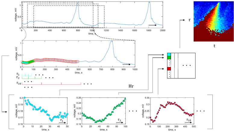
It could be noted that the use of enables to obtain a number of vectors which are joined to the matrix . The matrix essentially is a representation of the H-rank in different scales of the reconstructed signal being changed in time. The matrix is a two-dimensional feature of the segment of ECG. It both evaluates the algebraic complexity of the signal and visualizes its change in time. This concept is very close to the spectrogram approach where the Fourier spectrum is visualized in columns and the rows represent time or vice versa. For this reason we coin our two-dimentional feature as H-rankgram.
The algorithm of the proposed approach is depicted in Fig. 1. While estimating H-ranks, in this paper we fix machine epsilon 2.2×10⁻¹⁶ and limit maximum rank by 30.
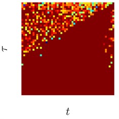
Some typical features extracted from the healthy and ill patient’s data are shown in Fig. 2. Note that the numerical values in each feature pattern is linearly transformed to the interval [0, 1]. In this way, patterns which are unusually bright or exceptionally dark are normalized. Thus the geometrical shapes in the feature pattern are preserved, but the numerical values become bounded and in turn more suitable for the input of neural networks.
3.3. On the proof of concept for the technique
The technique proposed is based on the rank of linear recurrence sequence (LRS). By investigating an ECG one assumes that it is LRS. But, of course, real-world sequences do not have a rank due to the presence of random noise. So the concept of pseudorank is introduced.
Suppose ECG as noisy LRS experiences a change in the dynamics. This in turn might and often will change the rank. Being a part of the H-rankgram the rank induces a visual change in the extracted 2D feature pattern. This euristic argument ensures that if algebraic complexity of the ECG is changing it will be noticeable in the feature pattern (if not visually then in the actual numerical values). This is the proof of the concept of the proposed algorithm.
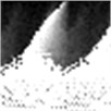
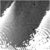
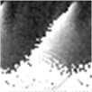
Fig. 22D feature patterns for healthy patients (parts (a)-(c)), and ill patients (myocardial infarction, parts (d), (f)). White color corresponds to maximum H-ranks while black depicts minimal H-ranks in the observation window
a)
b)
c)
d)
e)
f)
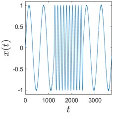
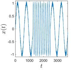
Sometimes algorithms are tested on trivial data to show that they actually work. We use here a time series comprised of 3 concatenated sinusoids: , , and to demonstrate that H-rankgram reflects a change in the dynamics of the underlying data. This concatenated time series is also contaminated with additive Gaussian noise to demonstrate the robustness of the algorithm.
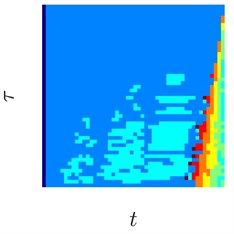
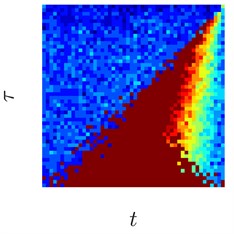
Fig. 3 clearly depicts that H-ranks for moving windows gradually reacts to the inclusion of the second sinusoid which is of different frequency. The amount of additive noise even strengthens this effect. This could be explained by the fact that there are more possible values for H-ranks for noisy sequences (they are usually higher in that case). But if the noise is high enough, the ranks will be also noticeably higher. And for completely random infinite sequence the rank is infinite.
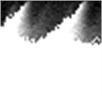
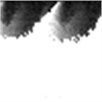
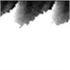
Fig. 3Sinusoids with different amount of additive Gaussian noise are depicted in parts (a)-(c). part (a) corresponds to the case of no noise. Parameters for the noise intensity are μ=0 and σ1=0, σ2=0.01, σ3=0.05 correspondingly. Parts (d)-(f) show H-rankgrams for each of the sinusoid
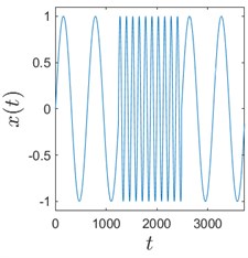
a)
b)
c)
d)
e)
f)
This simple numerical experiment supports the aforementioned euristic argument. Also, it shows that H-rankgram is robust to additive noise to a certain degree. Maximum tolerable amount of additive noise is another question and out of the scope of this paper.
3.4. Artificial neural network architectures used
As the main problem solved here is image classification we have used CNN and ResNet neural networks which are dedicated for solving exactly that type of problem. In general there is no particular method which could suggest the exact architecture of the network. Thus we performed a number of numerical experiments to determine the optimal number of layers as well as parameters for the filters. The experiments are summarized in the next section.
Usually 2-3 convolutional layers in CNN are sufficient for image classification task. So we have tested 2 to 4 layers. As for filter sizes, 2×2 to 5×5 were tested. The number of filters were also optimized by testing different variants. The best architectures are discussed in the next section. As for ResNet, same number of filters were tested, but only 2 and 3 residual blocks were considered. Note that ResNet is an improved version of CNN incorporating skip connections which acts as a dropout approach, but applied to the whole convolutional layer.
Software coding of artificial neural networks were done by using Python and Tensorflow with Keras.
Fig. 4Architectures of CNN (part (a)) and ResNet (part (b)) used for classification of 2D features. Images generated by Netron software [23]
![Architectures of CNN (part (a)) and ResNet (part (b)) used for classification of 2D features. Images generated by Netron software [23]](https://static-01.extrica.com/articles/22138/22138-img14.jpg)
a)
![Architectures of CNN (part (a)) and ResNet (part (b)) used for classification of 2D features. Images generated by Netron software [23]](https://static-01.extrica.com/articles/22138/22138-img15.jpg)
b)
4. Experimental results
As described in Section 2.2 the problem solved here is to classify 2D feature patterns with respect of different ECG types. Of course, one can guess filter sizes and numbers by looking at the patterns of the images but usually we need to test a number of options and pick the best scenario. So it is almost a full sorting problem. A set of possible values for these parameters were mentioned in Section 3.4 and the top best results are summarized below. All the classification problems were repeated 64 times, each time randomly selecting 70 % of the images from each class for training and 30 % of the images for validation. This is in order to reduce the variance of the estimated accuracy. The random part also acts as cross validation of the modelling.
Table 1Average classification accuracy for 9 classes of ECG feature patterns. The modelling was repeated 64 times. The bold values shows the best architecture of the neural network
CNN | ||||
Filter sizes | Convolutional layers | Number of filters | Average accuracy | |
Training | Validation | |||
2 | 3 | [8 16 32] | 0.7127 | 0.6931 |
3 | 3 | [8 16 32] | 0.7137 | 0.6924 |
2 | 3 | [11 22 33] | 0.7128 | 0.6934 |
2 | 3 | [9 11 18] | 0.7117 | 0.6936 |
ResNet | ||||
Filter sizes | Residual blocks | Number of filters | Average accuracy | |
Training | Validation | |||
2 | 2 | [16 32 64] | 0.8255 | 0.6938 |
2 | 3 | [16 32 64 128] | 0.9980 | 0.6938 |
3 | 3 | [16 32 64 128] | 0.9991 | 0.6938 |
4 | 2 | [16 32 64] | 0.9363 | 0.6938 |
Table 2Average sensitivity and specificity for the investigation of 9 classes of ECG feature patterns using optimal CNN and ResNet networks. The modelling was repeated 64 times
ANN | No. classes | Sensitivity | Specificity |
CNN | 9 | [0 0 0 0 0 0.9994 0 0.0013 0] | [1 1 1 1 1 0.0022 1 0.9990 1] |
ResNet | 9 | [0 0 0 1 0 0 0 0 0] | [1 1 1 0 1 1 1 1 1] |
Table 1 shows that on average ResNet gives better accuracy while working with 9 classes of feature patterns (0.6938 versus 0.6936). One can observe that accuracy in the validation set is very similar between different neural network architectures. This is mainly the result of some classes containing just a few items.
In this paper we have used one against all approach to estimate sensitivity and specificity for multi-class classification problem. Sensitivity estimates of the classification problem for CNN and ResNet approaches (Table 2) are not evenly distributed between the classes. As for CNN, the feature patterns are always assigned to class 6 (Myocardial infarction) or 8 (Healthy control), but for ResNet the patterns are assigned to class 4 (Valvular heart disease). This suggests that smallest peculiarities of the feature patterns does not need to be considered for classification. CNN, being of lower capabilities to memorize smaller objects compared to ResNet, outperformed the latter.
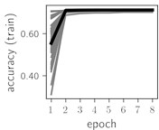
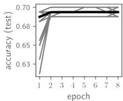
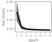
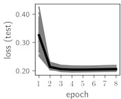
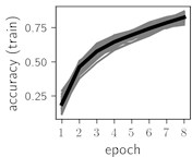
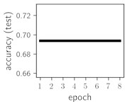
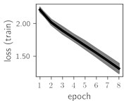
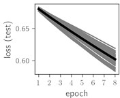
Fig. 5Training dynamics for CNN (parts (a)-(d)) and ResNet (parts (e)-(h)) neural networks with 9 classes of ECG feature patterns. CNN was comprised of 3 convolutional layers with 9, 11 and 18 2×2 filters. ResNet was comprised of 2 residual blocks with 16 and 32 as well as 32 and 64 2×2 filters
a)
b)
c)
d)
e)
f)
g)
h)
Considering the training dynamics (Fig. 5) with 9 classes of ECG feature patterns, supremacy of the CNN architecture is more emphasized. One can observe that the training process stabilizes in both training and testing samples as early as at epoch 3. On the contrary, ResNet overfits (accuracy in the training set keeps increasing but it is stable at the testing set) right after the first epoch. Furthermore, the loss function (categorical or binary cross entropy depending on the number of classes considered) keeps to decrease at epoch 8. The modelling was repeated 64 times and we can note that each time training dynamics was similar – this shows a high stability of the results.
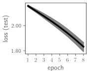
As we can see in the Table 3, average classification accuracy in the training set as well as in the validation set using only 2 classes is greater compared to the average classification accuracy having 9 classes. Comparing two artificial neural networks, ResNet is more accurate than CNN in the validation set (0.8222 versus 0.8219). Thus, the best classification experiments, either choosing 2 or 9 classes, are both the same with respect of their filter sizes (2), residual blocks (2), convolutional layers (3) and the number of filters (9, 11 and 18 for the CNN and 16, 32 and 64 for the ResNet). It could be mentioned that the results obtained do not strongly depend on the type of artificial neural network. It also suggests that lower complexity neural networks could be employed for the classification task of feature patterns extracted.
Table 3Average classification accuracy having 2 classes of ECG feature patterns. The modelling was repeated 64 times. The bold values show the best architecture of the neural network
CNN | ||||
Filter sizes | Convolutional layers | Number of filters | Average accuracy | |
Training | Validation | |||
2 | 3 | [8 16 32] | 0.8212 | 0.8218 |
3 | 3 | [8 16 32] | 0.8215 | 0.8219 |
2 | 3 | [11 22 33] | 0.8211 | 0.8215 |
2 | 3 | [9 11 18] | 0.8209 | 0.8219 |
ResNet | ||||
Filter sizes | Residual blocks | Number of layers | Average accuracy | |
Training | Validation | |||
2 | 2 | [16 32 64] | 0.9500 | 0.8222 |
2 | 3 | [16 32 64 128] | 0.9920 | 0.8222 |
3 | 3 | [16 32 64 128] | 0.9883 | 0.8222 |
4 | 2 | [16 32 64] | 0.9799 | 0.8222 |
Table 4Average sensitivity and specificity for the investigation of 2 classes of ECG feature patterns using optimal CNN and ResNet networks. The modelling was repeated 64 times
ANN | No. classes | Sensitivity | Specificity |
CNN | 2 | [0.9994 0.0007] | [0.0007 0.9994] |
ResNet | 2 | [0 1] | [1 0] |
Table 4 shows that in the case of only 2 classes again CNN was able to distinguish the feature patterns better between the classes. Same as in the previous case with 9 classes, features patterns corresponding to Myocardial infarction are detected with greater accuracy compared to other types of patterns. In the practical applications this would not necessary be an unwanted feature. It might be safer to raise a red flag than to ignore an important illness.
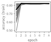
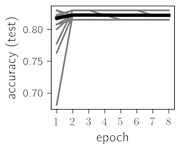
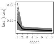
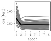
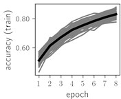
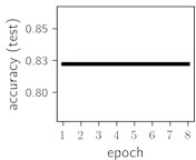
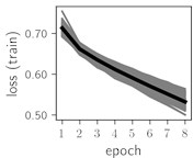
Fig. 6Training dynamics for CNN (parts (a)-(d)) and ResNet (parts (e)-(h)) neural networks with 2 classes of ECG feature patterns. CNN was comprised of 3 convolutional layers with 9, 11 and 18 2×2 filters. ResNet was comprised of 2 residual blocks with 16 and 32 as well as 32 and 64 2×2 filters
a)
b)
c)
d)
e)
f)
g)
h)
Classification of feature patterns with 2 classes results in a very similar average training dynamics as with 9 classes also (Fig. 6). The only difference here is a slightly bigger spread of the accuracy and loss functions about their corresponding average values. Despite this result the overall classification accuracy is higher with 2 classes of feature patterns. This could be naturally expected as the classification complexity is smaller for lower number of classes.
5. Conclusions
H-rankgram as feature extraction method resulted in detecting Myocardial infarction more accurately compared to other classes of ECG. But important notice here is that the accuracy is low for feature patterns representing other types of ECG. In general, ECG might not be the best data to analyze with H-rankgrams. Note that often professionals look at ECG as a set of intervals between particular positions in the signal. The H-rankgram focuses on changes in algebraic complexity of the signal analyzed. Changes in values of those intervals might not necessary go along with the changes in algebraic complexity.
It was demonstrated that H-rankgram is robust to additive noise. This is an important property, since real-world signals such as ECG are susceptible to natural and systematic noise.
More advanced neural networks like ResNet typically have large number of parameters to be trained. CNN in this regard is generally much smaller network. The data set used contained only 521 records which is a very small number considering the dimension of the parameter space of the target function of the neural networks used. This is a natural limitation of this research with respect of the classification accuracy. Accuracy of 0.6938 with 9 classes and of 0.8222 with 2 classes still looks reasonable in this context.
References
-
R. R. Sharma, M. Kumar, and R. B. Pachori, “Joint time-frequency domain-based CAD disease sensing system using ECG signals,” IEEE Sensors Journal, Vol. 19, No. 10, pp. 3912–3920, May 2019, https://doi.org/10.1109/jsen.2019.2894706
-
X. Chen, J. Lin, C. Huang, and L. He, “A novel method based on adaptive periodic segment matrix and singular value decomposition for removing EMG artifact in ECG signal,” Biomedical Signal Processing and Control, Vol. 62, p. 102060, Sep. 2020, https://doi.org/10.1016/j.bspc.2020.102060
-
M.-B. Hossain, S. K. Bashar, J. Lazaro, N. Reljin, Y. Noh, and K. H. Chon, “A robust ECG denoising technique using variable frequency complex demodulation,” Computer Methods and Programs in Biomedicine, Vol. 200, p. 105856, Mar. 2021, https://doi.org/10.1016/j.cmpb.2020.105856
-
G. Wang et al., “ECG signal denoising based on deep factor analysis,” Biomedical Signal Processing and Control, Vol. 57, p. 101824, Mar. 2020, https://doi.org/10.1016/j.bspc.2019.101824
-
R. R. Sharma and R. B. Pachori, “Baseline wander and power line interference removal from ECG signals using eigenvalue decomposition,” Biomedical Signal Processing and Control, Vol. 45, pp. 33–49, Aug. 2018, https://doi.org/10.1016/j.bspc.2018.05.002
-
R. R. Sharma and R. B. Pachori, “Eigenvalue decomposition of hankel matrix-based time-frequency representation for complex signals,” Circuits, Systems, and Signal Processing, Vol. 37, No. 8, pp. 3313–3329, Aug. 2018, https://doi.org/10.1007/s00034-018-0834-4
-
D. P. Tobon and T. H. Falk, “Adaptive spectro-temporal filtering for electrocardiogram signal enhancement,” IEEE Journal of Biomedical and Health Informatics, Vol. 22, No. 2, pp. 421–428, Mar. 2018, https://doi.org/10.1109/jbhi.2016.2638120
-
N. Prashar, M. Sood, and S. Jain, “Design and implementation of a robust noise removal system in ECG signals using dual-tree complex wavelet transform,” Biomedical Signal Processing and Control, Vol. 63, p. 102212, Jan. 2021, https://doi.org/10.1016/j.bspc.2020.102212
-
K. Kærgaard, S. H. Jensen, and S. Puthusserypady, “A comprehensive performance analysis of EEMD-BLMS and DWT-NN hybrid algorithms for ECG denoising,” Biomedical Signal Processing and Control, Vol. 25, pp. 178–187, Mar. 2016, https://doi.org/10.1016/j.bspc.2015.11.012
-
P. Janbakhshi and M. B. Shamsollahi, “ECG-derived respiration estimation from single-lead ECG using gaussian process and phase space reconstruction methods,” Biomedical Signal Processing and Control, Vol. 45, pp. 80–90, Aug. 2018, https://doi.org/10.1016/j.bspc.2018.05.025
-
S. K. Mukhopadhyay and S. Krishnan, “A singular spectrum analysis-based model-free electrocardiogram denoising technique,” Computer Methods and Programs in Biomedicine, Vol. 188, p. 105304, May 2020, https://doi.org/10.1016/j.cmpb.2019.105304
-
S. K. Bashar, Y. Noh, A. J. Walkey, D. D. Mcmanus, and K. H. Chon, “VERB: VFCDM-based electrocardiogram reconstruction and beat detection algorithm,” IEEE Access, Vol. 7, pp. 13856–13866, 2019, https://doi.org/10.1109/access.2019.2894092
-
H. Hao et al., “Multi-lead model-based ECG signal denoising by guided filter,” Engineering Applications of Artificial Intelligence, Vol. 79, pp. 34–44, Mar. 2019, https://doi.org/10.1016/j.engappai.2018.12.004
-
F. Ertuğrul, E. Acar, E. Aldemir, and A. Öztekin, “Automatic diagnosis of cardiovascular disorders by sub images of the ECG signal using multi-feature extraction methods and randomized neural network,” Biomedical Signal Processing and Control, Vol. 64, p. 102260, Feb. 2021, https://doi.org/10.1016/j.bspc.2020.102260
-
M. Benouis, L. Mostefai, N. Costen, and M. Regouid, “ECG based biometric identification using one-dimensional local difference pattern,” Biomedical Signal Processing and Control, Vol. 64, p. 102226, Feb. 2021, https://doi.org/10.1016/j.bspc.2020.102226
-
M. Hammad, S. Zhang, and K. Wang, “A novel two-dimensional ECG feature extraction and classification algorithm based on convolution neural network for human authentication,” Future Generation Computer Systems, Vol. 101, pp. 180–196, Dec. 2019, https://doi.org/10.1016/j.future.2019.06.008
-
M. Hammad, G. Luo, and K. Wang, “Cancelable biometric authentication system based on ECG,” Multimedia Tools and Applications, Vol. 78, No. 2, pp. 1857–1887, Jan. 2019, https://doi.org/10.1007/s11042-018-6300-2
-
B. M. Mathunjwa, Y.-T. Lin, C.-H. Lin, M. F. Abbod, and J.-S. Shieh, “ECG arrhythmia classification by using a recurrence plot and convolutional neural network,” Biomedical Signal Processing and Control, Vol. 64, p. 102262, Feb. 2021, https://doi.org/10.1016/j.bspc.2020.102262
-
A. S. Eltrass, M. B. Tayel, and A. I. Ammar, “A new automated CNN deep learning approach for identification of ECG congestive heart failure and arrhythmia using constant-Q non-stationary Gabor transform,” Biomedical Signal Processing and Control, Vol. 65, p. 102326, Mar. 2021, https://doi.org/10.1016/j.bspc.2020.102326
-
G. Petmezas et al., “Automated atrial fibrillation detection using a hybrid CNN-LSTM network on imbalanced ECG datasets,” Biomedical Signal Processing and Control, Vol. 63, p. 102194, Jan. 2021, https://doi.org/10.1016/j.bspc.2020.102194
-
Goldberger et al., “PTB Diagnostic ECG Database.” https://physionet.org/content/ptbdb/1.0.0/, 2004.
-
M. Ragulskis and Z. Navickas, “The rank of a sequence as an indicator of chaos in discrete nonlinear dynamical systems,” Communications in Nonlinear Science and Numerical Simulation, Vol. 16, No. 7, pp. 2894–2906, Jul. 2011, https://doi.org/10.1016/j.cnsns.2010.10.008
-
Lutz Roeder, “Netron.” GitHub repository. https://github.com/lutzroeder/netron
About this article

