Abstract
Due to the limitation of working environment and structure conditions, it is difficult to directly measure the propeller excitation of ship propulsion shafting system. A method based on waveguide function and modal method combining with shafting vibration response measurement was proposed to estimate the propeller longitudinal excitation indirectly. Firstly, a waveguide transfer model for the general structure of the propulsion shafting is proposed that is suitable for estimating propeller excitation from shafting vibration response. Secondly, the longitudinal excitation of the propeller is calculated by measuring the waveguide coefficients of any shaft sections via the proposed hybrid method. Finally, the scheme is verified by a concrete example. The simulation results prove its feasibility and effectiveness for estimating propeller excitation by measuring the shafting vibration response, which provides a novel scheme for accurately grasping the propeller excitation and effectively controlling the vibration and noise of hull structure.
1. Introduction
The propeller excitation force is an essential exciting source for submarine underwater navigation. When the propeller runs in a temporally varying and spatially uneven flow field near the stern of the submarine, the hull can be excited to produce noise radiation by the unsteady dynamic force caused by the non-uniform force on each blade, which has an important impact on the underwater acoustic stealth performance of the submarine [1]. How to simulate the real stern flow conditions and the study of the scale effect and similarity between the experimental model and the real model are essential to accurately predicting the direct noise of the propeller.
Due to the limitations of the working environment and structural conditions, the propeller excitation of the marine propulsion shafting is difficult for direct measurement [2]. The spectrum of the unsteady force of the propeller is composed of the spectrum of the low-frequency discrete force with the blade-passing-frequency (BPF) and double-BPF generated by the uneven force on the blades, and the spectrum of the low-frequency broadband force generated by the interaction between the stern turbulence and the propeller, which can be obtained mainly through experimental tests, semi-empirical formulas [3], and numerical calculations [4]. In the test pool, the scaled model can be measured to obtain the spectrum of the unsteady force of the propeller, but the correlation between the test results and the real ship model is still unclear. Besides, the lateral force measurement is more complicated, and no effective measurement means have been established yet. The numerical calculation of the spectrum of the low-frequency discrete force mainly includes the lifting surface method, panel method, and CFD method, etc. [5]. In the lifting surface method, the blade is assumed as a thin wing to calculate the pressure distribution of the blade, but the influence of the hub is not taken into consideration. In the panel method, the calculation of the propeller excitation force can reflect the actual operating conditions of the propeller to the greatest extent, the influence of the hub is taken into account, more accurate calculation results can be obtained, and there is no need for the thin wing hypothesis [6, 7]. Based on the software Fluent for fluid mechanics computation, Ma Chao applied the RNG turbulence model to analyze the uneven turbulent flow near the propeller and the non-uniform pressure pulsation near the propeller under the influence of the turbulent flow. The author also studied the variation of the bearing force and moment of the propeller [8]. It is difficult to calculate the low-frequency broadband force spectrum of the propeller. Some software for fluid computation can be used to theoretically simulate and analyze the propeller excitation in the flow field, or building a physical model of the shafting in the laboratory to conduct experimental research on the propeller excitation characteristics. Still, they are different from the real shaft system. Therefore, grasping the propeller excitation under actual working conditions is very important for maneuvering the vibration and noise of the propeller and propulsion shafting, and controlling the vibration of the hull structure caused by the shafting vibration.
According to the dynamics theory, the excitation can also be estimated by measuring the vibration response of the system when the real excitation cannot be measured, which belongs to the second type of inverse problem of the dynamics [9]. Since it is difficult to directly measure the fluid excitation of the propeller in working conditions in seawater, it becomes a reasonable choice to estimate the propeller excitation by measuring the vibration response of the shafting. This estimation must be carried out on the premise that the vibration model of the shafting has been established. Therefore, a theoretical model for estimating the excitation of the propeller from the shaft vibration response should be first established based on the general structure of the propulsion shafting. However, there exist some practical difficulties in dealing with the above problem solely by the modal theory, for examples:
1. It is not easy to arrange a large number of vibration sensors on the entire shafting, especially the stern section close to the propeller. Therefore, it is almost impossible to fully grasp the actual vibration of the shafting through the vibration response measurement.
2. Although it is technically feasible to establish a finite element model (FEM) based on the structural size and material properties of the shafting, the determination of the boundary conditions of the shafting is difficult, especially for the shaft-hull connections with thrust bearings. There is currently a lack of reliable theoretical calculations or measurement methods for the parameters, including the longitudinal oil film stiffness of the thrust bearing and the admittance of the joint structure between the thrust bearing housing and the hull.
Based on the waveguide theory, the waveguide model of different shaft sections of the shafting and the waveguide transfer relationship between the connected shaft sections are established in response to the above difficulties. Assuming there is a shaft section suitable for direct vibration response measurement. The waveguide coefficient can be estimated based on the vibration response observation data of the shaft section and the pre-established shaft section waveguide model. The longitudinal excitation of the propeller can be derived from the waveguide model of the shaft section and each connecting shaft section of the propeller and the waveguide transfer relationship between these connecting shaft sections. Since the waveguide model and the vibration response observation data of the shaft section are used to estimate the waveguide coefficients, the boundary conditions of the shaft section are not involved, so the estimation of the longitudinal oil film stiffness of the thrust bearing and the admittance of the joint structure between the thrust bearing housing and the hull are avoided. At the same time, after the waveguide model of the entire shafting is established, the method for estimating the waveguide coefficient of a shaft section using the vibration response can also be used to calculate the longitudinal excitation from the shafting to the hull through the thrust bearing, which is the same as the principle of estimating the longitudinal excitation of the propeller. Based on this, the admittance function test problem of thrust bearing housing can also be discussed.
2. Basic principle
2.1. Theoretical model construction
The unsteady force generated by the propeller in the non-uniform wake field at the stern of the hull, the radial simple harmonic component force generated by the main engine device and the longitudinal component force generated by the torsional vibration of the propulsion shafting all make the propulsion shafting produce periodic longitudinal tension and compression deformation, which is the common longitudinal vibration of the propulsion shafting of large ships and submarines. The analysis of the longitudinal vibration mechanism of propulsion shafting focuses on solving two problems: one is to calculate the longitudinal vibration characteristics of propulsion shafting and its influencing factors, and to judge whether there is longitudinal resonance of propulsion shafting within the normal speed range of the main engine; The second is to analyze the longitudinal dynamic response of the typical excitation of the propulsion shafting, and judge whether the response amplitude is within the allowable range, so as to avoid the adverse effects of the secondary excitation force generated by the longitudinal vibration of the shafting on other structures of the hull.
Fig. 1 is a general multi-shaft (rod) section longitudinal vibration model based on the general structure of the shafting, wherein the propulsion shafting is assumed to consist of uniform shaft sections, and , , , …, represent coordinates of the endpoint of the shaft (rod) sections. Note that the length of the -th (1, 2, …, ) shaft (rod) section is , and the cross-sectional area is . Each rod section has a complex elastic modulus of and a density of . The mass of the propeller is . The coupling stiffness between the shafting and the hull (thrust bearing axial stiffness) is . The admittance in the longitudinal vibration direction of the joint position between the shafting and the hull is . The longitudinal excitation of the propeller is .
Fig. 1Simplified model of the longitudinal vibration of the propulsion shafting
Let represent the longitudinal vibration displacement of the particle on the shaft, and it satisfies the following wave function and boundary conditions:
By measuring the longitudinal vibration response of the shafting, the longitudinal excitation of the propeller can be estimated mainly based on the following considerations:
(1) Lack of direct measurement means for the longitudinal excitation of the propeller;
(2) For real systems, the connection stiffness is generally not easy to be determined;
(3) The relevant geometric parameters and material characteristic parameters of each shaft section and the propeller of the propulsion shafting can be accurately obtained;
(4) The longitudinal vibration response of the shaft system can be directly measured.
Let represent the vibration displacement of each shaft section, then:
where represents the Fourier transform of and the section stiffness is given by .
The waveguide method [10] is adopted to establish the shaft model (as shown in Fig. 1), and each shaft section is described by wave solution :
where is the complex wavenumber, and . At the far left end (set 0), the boundary conditions are given by:
Substitute Eq. (3) into Eq. (4), then we have:
Therefore, if and are measurable or identifiable, the longitudinal excitation of the propeller can be calculated by the above equation. Now suppose that or of the first shaft section at the left side can be measured arbitrarily, then arrange several measuring points on the shaft at the location of , , , …, , we get:
where, presents the measurement error. These measuring points are presented as a matrix expression:
Applying the principle of least square estimation, the residual expression is:
Let:
we have:
Using the above equation to estimate and requires 2. When the shaft section is simplified to a uniform cross-section structure and the model parameters are accurate, Eqs. (5), (7), and (10) can be used to calculate the longitudinal excitation of the propeller. Because theoretical derivation is rigorous, there is no need for verification with specific examples. However, since the real shafting system usually has many structures such as key grooves, local bumps, and external coating materials, various degrees of simplification are needed in the simplifying process of the shaft section into an ideal homogeneous, uniform cross-section waveguide model, which will introduce theoretical calculation errors. In addition, the measurement of vibration response will also generate errors. To reduce the impact of measurement errors, the least square estimation algorithm of Eq. (10) is adopted.
2.2. The problem wherein measuring points cannot be arranged on the shaft section close to the propeller
The method of using Eqs. (5), (7), and (10) to estimate the longitudinal excitation of the propeller from the measured longitudinal vibration response does not require the parameters of the other connecting shaft sections after the first shaft section in Fig. 1, and the longitudinal stiffness of the thrust bearing of the right side of the shafting and housing admittance parameters, which is the convenience of the above method. However, in practical applications, it may be challenging to arrange sensors on the stern section of the shafting close to the propeller to measure the longitudinal vibration response. Therefore, it is necessary to further consider picking up the longitudinal vibration response on the shaft section close to the thrust bearing to verify the feasibility of the indirect estimation of the longitudinal excitation of the propeller.
It is still assumed that each shaft section is a constant-section structure, and its longitudinal vibration response is expressed by Eq. (3). At the junction of any -th section and its left ()-th section (2), there are continuity conditions for displacement response and internal force, namely:
Substitute Eq. (3) into the above equation, we have:
That is:
So:
Therefore, if the and of the -th shaft section are measurable, then the and of the ()-th shaft section are calculated from the above formula. Using this recurrence relationship, and can be derived. Finally, substitute and into Eq. (5) to estimate the longitudinal excitation .
For the measurement of and , the least square estimation method of Eq. (10) is still used, namely:
where is a column vector composed of the longitudinal vibration response at 2 measuring points arranged on the -th shaft section. Refer to Eq. (7), can be written as:
It should be pointed out that the application of the above recursive algorithm requires as much as possible to ensure the accuracy of the waveguide model of the measurable shaft section and that on its left side up to the propeller. In actual operation, approximating parameters in the waveguide model will cause calculation errors in each recursive calculation, and the errors will be accumulated during multiple recursions. Therefore, the arrangement of measuring points on the shaft far away from the propeller will increase the uncertainty in theoretical calculations and reduce the estimation accuracy of the propeller excitation. Although the recursive algorithm is theoretically feasible, the measuring points should be arranged as close as possible to the longitudinal excitation shaft section.
3. Measuring waveguide coefficients of any shaft section by combining waveguide method and modal method
The general longitudinal vibration displacement of the shafting is described by Eq. (3). Its calculation accuracy depends entirely on the calculation accuracy of the section stiffness and wavenumber , that is, the accuracy of the physical model of the shafting. As for determining the waveguide coefficients of and , it can boil down to the initial value problem of the differential equation of Eq. (4). As long as the accuracy of the initial value and the physical model of the shafting is sufficient, the obtained waveguide coefficients can be guaranteed to have enough calculation accuracy. Lastly, Eq. (14) describes the conversion relationship of the waveguide coefficients when each shaft section of the shafting has a uniform cross-section. The calculation accuracy also completely depends on the physical modeling accuracy of the shafting. Therefore, the longitudinal excitation of the propeller can be estimated using the above-mentioned waveguide transfer model if the waveguide coefficients of some section of the shafting are given.
For the forward problem of dynamics, the complete solution of the shaft waveguide model requires clear boundary conditions and external excitation [11]. However, to calculate the propeller excitation problem from the measured shaft vibration response, it must be assumed that the vibration response of a certain section of the shafting can be measured, and the waveguide coefficients of the shaft section can be estimated through the measured response, so the boundary conditions of the waveguide model are not necessary, which allows unknown at the right end of the shafting (Fig. 1) and admittance in the longitudinal vibration direction at the connection between the thrust bearing housing and the hull. The basic principle of combining the waveguide method and the modal method to measure the waveguide coefficients of any shaft section is to identify the influence factors of the main vibration modes through the arrangement of as few measuring points as possible, then apply the modal superposition theory to fit the analytical expression of curve, and finally calculate on this basis. The detailed steps are as follows:
Firstly, the shaft section to be measured is a certain part of the entire shafting. Separating the shaft section in the entire shafting, that is, releasing the constraints of other shaft sections or structures in the shafting to the shaft section to be measured and replacing them with binding forces and . The shaft section to be measured is regarded as a free rod at both ends, and and are regarded as the external excitation. Even the longitudinal vibration mode of this shaft section is not accessible for theoretically calculation; its numerical solution can be easily obtained through accurate finite element modeling, that is, when the shaft section to be measured is regarded as a free rod at both ends, its longitudinal vibration mode is easy to be determined with guaranteed accuracy.
Let represent the mode function of each order of the longitudinal vibration of the measured shaft section. By using the modal superposition theory, we get:
where, and represent the modal quality and modal frequency of the shaft section, respectively; is the damping loss factor; represents the impact factor (weight factor) of the -th mode when the modal superposition is used to synthesize .
Suppose that observation points of , , …, are taken from the shaft section. The measured values of longitudinal vibration response are , , …, , and according to Eq. (17) the measured value of each observation point can be expressed as the following matrix equation:
where , , …, represent the modal truncation error generated when , …, are synthesized with the -order low-frequency modes, and the measurement error in the actual observation value , , …, . In fact, it is the core of the problem to estimate the low-frequency components in the longitudinal excitation of the propeller, and the natural frequencies of the shaft sections are generally relatively high. For example, for a 1-m steel shaft with a uniform cross-section, a free boundary at both ends, except for the modal frequency of its rigid body 0, the lowest non-zero natural frequency is 2594.4 Hz. Therefore, even the impact factors of the first two modes (presumably designing the first three low-frequency modes, including the rigid body mode) in the low-frequency band are included, it can be assured the modal truncation error is within a smaller order of magnitude. In the real test analysis, the main component of the error vector will be the measurement error.
In order to eliminate the influence of the error vector as much as possible, the least square estimation principle is applied to Eq. (18) to estimate the modal influence factor, and we have:
The modal influence factor can be estimated with Eq. (19). Generally, multiple observation points should be arranged in a scattered manner, and the number is larger than that of main influencing modes, i.e., . The more observation points there are, the higher the confidence in the estimation of . For estimating the low-frequency longitudinal excitation of the propeller, as mentioned above, it is usually sufficient to consider the first three low-frequency modes including the rigid body mode, that is, the number of observation points 3, which is relatively easy to achieve in the real test. Besides, care should be taken to avoid placing the observation point on (or near) the node of the main influencing mode, because this will lead to the impact factor of this mode cannot be truthfully reflected in the observation data.
After the impact factor of the primary influencing mode is estimated, the response function and the slope function of the shaft section to be measured can be expressed as:
where represents the estimated value of the impact factor (the -th element of ) of the -th primary influencing mode.
Substitute the above equation into Eq. (20), the we obtain the estimated value of the waveguide coefficients as:
where and are differential operators, with:
Finally, it must be pointed out that by the convergence theorem of Fourier series [12], Eq. (21) cannot be used to estimate the waveguide coefficient near the end of the rod; To do this, you should first estimate waveguide coefficient at the middle of the rod using Eq. (21), and then calculate the waveguide coefficient at the end with Eq. (14).
4. Examples
The following calculation examples are used to theoretically verify the method of estimating the waveguide model through modal superposition method.
Assume a round steel shaft (rod) with a uniform cross-section and both free ends with the length 1 m, radius 0.03 m, complex elastic modulus 210×109(1+0.01j) Pa, density 7800 kg/m3. Establish a one-dimensional coordinate system along the rod axis, and set 0 at the left end and at the right end.
4.1. The relationship between wave solution and modal superposition solution
Excitation and are applied onto the left and right end of the rod. The longitudinal vibration displacement of the rod satisfies the waveguide model of Eq. (2). Because rod cross-section is uniform, the waveguide coefficients and are independent of . According to the following boundary conditions:
the waveguide coefficient can be obtained as:
Substitute the above equation into Eq. (3), we get:
Extend the above equation into the following even function with a period of 2:
And then expand to a Fourier series, for , we have:
where:
Note that substituting Eqs. (27) and (28) into Eq. (26), we get the modal superposition equation, namely:
The first term of the above equation corresponds to the impact factor of the longitudinal vibration rigid body mode (natural frequency 0, mode type 1) of a uniform rod with free ends. According to Eq. (29), the (complex) natural frequency of the rest non-rigid body modes, mode type, and mode impact factor respectively are:
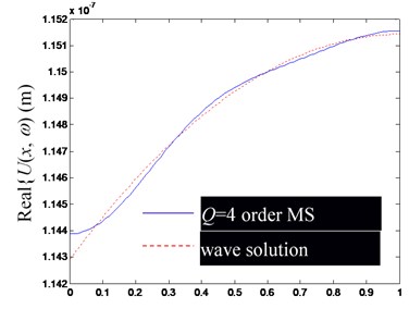
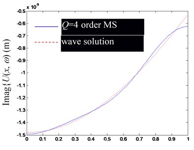
Therefore, for a uniform free rod excited from both ends, the wave solution (Eq. (24)) is an exact analytical solution, and the modal superposition solution (Eq. (28)) is the Fourier series expansion of the wave solution. If the excitation frequencies of and are low (generally lower than the first-order non-zero natural frequency of the rod), because the high-order mode has a small impact factor, the superposition synthesis with finite low-order modes is used to approximate . Figs. 2-4 show the comparison between the by superposition synthesis with the first -order modes (including rigid body modes) and its precise wave solution. It is assumed that (N) and (N). The excitation frequency of 100 Hz, 400 Hz, 1000 Hz is selected.
Fig. 2Comparison of Ux,ω by superposition synthesis with the first low-order modes (including rigid body mode) and their precise wave solutions (excitation frequency f= 100 Hz)
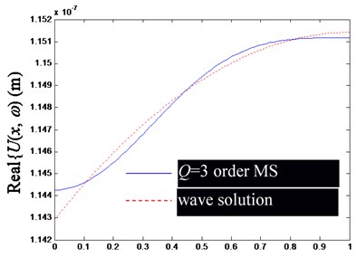
a) Real part of
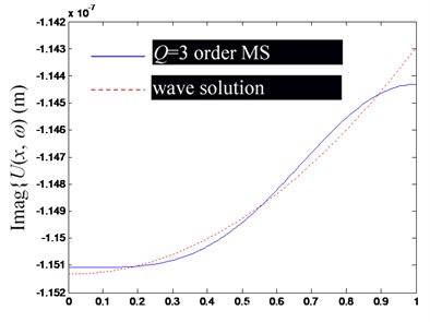
b) Imaginary part of
c) Real part of
d) Imaginary part of
Fig. 3Comparison of Ux,ω by modal superposition (MS) synthesis of the first low-order modes (including rigid body mode) and their precise wave solutions (excitation frequency f= 400 Hz)
a) Imaginary part of
b) Imaginary part of
c) Real part of
d) Imaginary part of
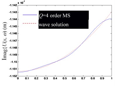
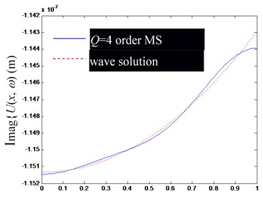
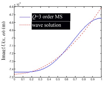
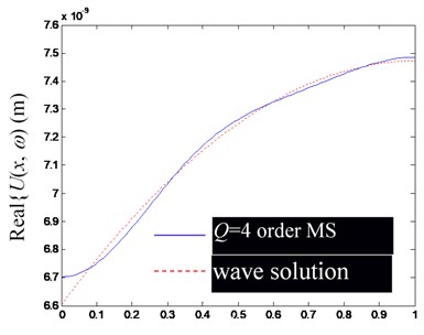
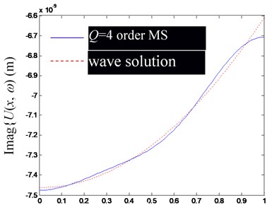
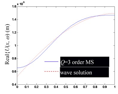
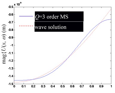
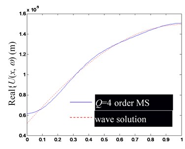
Based on the Figs. 2-4, in the low-frequency band, the consistency of by superposing several low-frequency modes and the precise wave solution is mainly determined by the mode order involved in modal superposition, but slightly affected by the change of excitation frequency. Obviously, the more modal orders involved in the modal superposition, the closer the result of modal superposition is to the exact wave solution.
Besides, notice that at the left and right ends of the rod, there are significant deviations between the finite modal superposition result and the exact wave solution (the point of 0 in (a) and (c), and in (b) and (d) in Figs. 2-4). It can be attributed to the usually discontinuous derivatives at 0 and , obtained by extending to get through Eq. (25). In fact, from the Fourier series solution of Eq. (29), there will be 0 at 0 and , but the wave solution of Eq. (24) does not lead to the same conclusion, which can be explained by referring to the convergence theorem of the Fourier series.
In summary, the accuracy of synthesized by superposing finite-order modes is mainly determined by the convergence of the Fourier series, which has a slower convergence speed at both ends of the rod.
Fig. 4Comparison of Ux,ω by superposition synthesis with the first low-order modes (including rigid body mode) and their precise wave solutions (excitation frequency f= 1000 Hz)
a) Real part of
b) Imaginary part of
c) Real part of
d) Imaginary part of
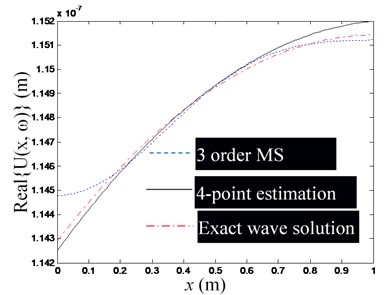
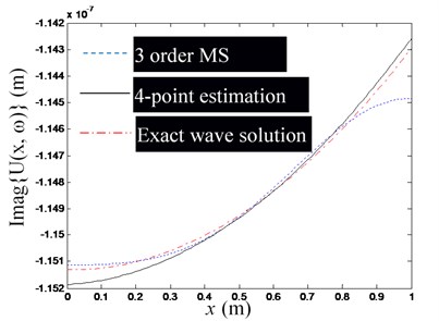
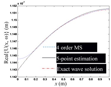
4.2. Estimating waveguide coefficients based on the vibration response data of finite observation points and modal function
Note that the obtained by the modal superposition method (Eq. (29)) cannot be used to calculate the end excitation and of the rod, because it does not satisfy Eq. (22). Therefore, in order to use the vibration response data of the limited observation points to invert the end excitation of the rod, the waveguide coefficients and must be first estimated, and then substituted into the wave solution of Eq. (3); finally, and can be calculated using Eq. (22). In addition, for the uniform cross-section rod in this example, Eqs. (7)-(10) can be used to estimate the waveguide coefficients. This method does not need to be studied through simulation examples. The following is mainly based on Eqs. (18)-(21) to estimate the waveguide coefficient by combining the waveguide method and the modal method.
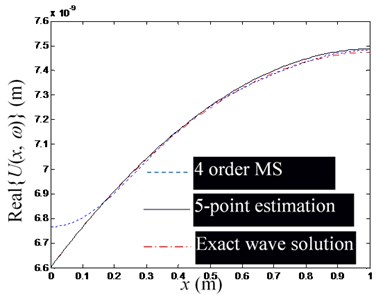
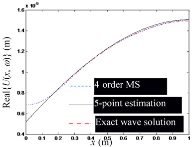
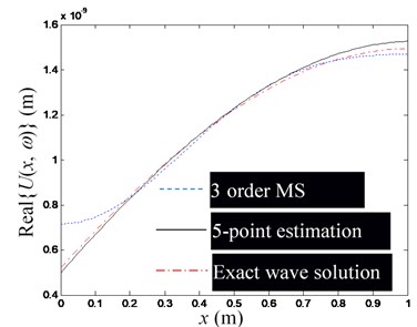
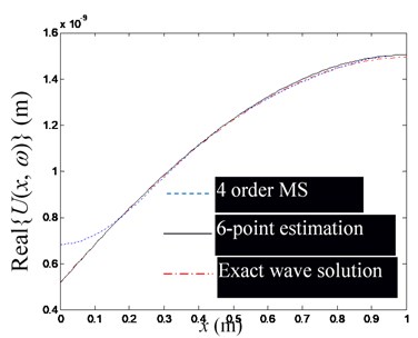
Fig. 5The influence of the number of mode superposition on the estimation accuracy of waveguide coefficients (Excitation frequency f= 100 Hz)
a) Real part of , at 4, 3
b) Imaginary part of , at 4, 3
c) Real part of , at 5, 4
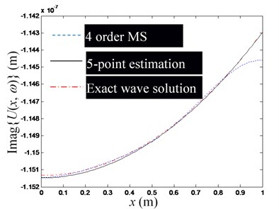
d) Imaginary part of , at 5, 4
e) Real part of , at 7, 6
f) Imaginary part of , at 7, 6
Firstly, as in Eq. (18), suppose that the first -order modes of the rod are used to synthesize , and arrange () observation points on the rod. Since the modal superposition series solution of converges slowly at the rod end, it is necessary to avoid arranging observation points close to the end of the rod; Temporarily select a section of 2/3 rod length from the middle of the rod for arranging the measurement points, and arrange the P observation points evenly.
Secondly, substitute the coordinate value of each observation point into Eq. (24), and calculate the longitudinal vibration response of each observation point as the theoretical simulation of the observation value to form the observation vector in Eq. (18). Substitute the coordinate value of each observation point into the mode function of Eq. (30), and then take the first -order mode function value to form the observation point mode type matrix of Eq. (18), and then estimate the mode impact factor vector by Eq. (19). Further substitute and the coordinate values of each observation point into Eq. (21) to estimate the waveguide coefficients and . Note that because rod cross-section is a uniform cross-section, the and should be constant in theory. But due to the calculation errors, the calculated waveguide coefficients corresponding to different observation points are different in practice, so the mean value of the estimated waveguide coefficients will be used as the final estimated value of and .
Finally, in the following Figs. 5-7, the exact wave solution of , -order modal superposition estimation and wave solution estimation based on the -order modal superposition estimation are compared to illuminate the feasibility of the proposed method for estimating the waveguide coefficients and the factors affecting the accuracy of the estimation results. The exact wave solution of is calculated by Eq. (24). The -order modal superposition estimation of is obtained by substituting the modal impact factor vector into the first equation of Eq. (20). The wave solution estimation based on the -order modal superposition estimation is calculated by substituting the estimated value of the waveguide coefficient into Eq. (3).
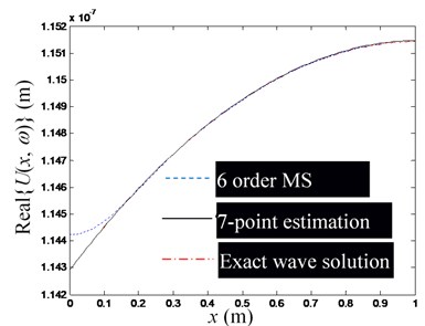
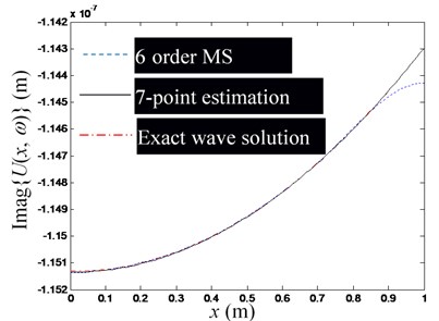
Fig. 6The influence of the change of excitation frequency (in the low-frequency domain) on the accuracy of waveguide coefficient estimation
a) Real part of , at 400 Hz
b) Real part of , at 1000 Hz
Fig. 5 shows a set of figures, indicating that the more modal orders included in the modal superposition, the higher the accuracy of the estimation of the waveguide mode; but as the modal order increases, its influence in the low-frequency domain decreases rapidly, thus for low-frequency problems, there is no need for too many modal orders. Since the required number of observation points is no less than the order of the mode participating in the superposition, and is used in Figs. 5(a)-(e). Fig. 6 shows that when the excitation frequency changes in the low-frequency band, the estimation accuracy of the waveguide model is marginally affected. Fig. 7 shows that when the number of modal orders is small, the estimation accuracy of the waveguide coefficient can also be increased by increasing the number of measuring points (Note that no matter the number of measuring points, you should avoid placing measuring points near the end of the rod). However, when the modal order is sufficiently large, the number of measurement points () has no significant effect on the estimation accuracy of the waveguide coefficient.
Fig. 7The influence of the number of observation points on the estimation accuracy of waveguide coefficients (Excitation frequency f= 1000 Hz)
a) Real part of , at 5, 3
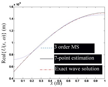
b) Real part of , at 7, 3
c) Real part of , at 6, 4
d) Imaginary part of , at 8, 4
5. Conclusions
The waveguide method is used to estimate the excitation of the propeller. Because there could be many intermediate transmission shaft sections between the measuring shaft section and the propeller, it is necessary to accurately describe the waveguide model of each shaft section and the transfer relationship between them. Based on the multi-section shaft model of Fig. 1, the obtained conclusions are summarized as follows:
1) If the shaft section connected with the propeller can be regarded as a uniform shaft section, and its longitudinal vibration response can be measured, the waveguide coefficients and can be simply estimated with Eqs. (7)-(10), and then the longitudinal excitation of the propeller can be calculated by using Eq. (5); Because the measuring point is close to the excitation position, this estimation displays high reliability.
2) In practice, when it is challenging to arrange sensors close to the stern section near the propeller, it is necessary to establish the waveguide model and the waveguide coefficient transfer relationship between the measuring shaft section and each shaft section connected to the propeller. And the propeller longitudinal excitation can be calculated by using Eqs. (5) and (14)-(16).
3) In multiple recursive calculations, the approximate processing of the parameters of the waveguide model can lead to the accumulation of calculation errors. Therefore, arranging measurement points far away from the shaft section near the propeller can reduce the estimation accuracy of the propeller excitation, and the measurement points should be arranged as close as possible to the shaft section near the propeller.
4) This work is limited to the theoretical demonstration of a hybrid method for estimating the longitudinal propeller excitation from the measured longitudinal vibration response. Because the theoretical derivation is rigorous, numerical simulation to verify the aforementioned method is no longer necessary, and its practical implementation is also feasible. However, designing a specific experimental system to conduct certain experimental research to clarify the specific influencing factors for errors in the actual excitation estimation is still valuable.
References
-
Ji Gang, Zhou Qidou, Tan Lu Coupling characteristic and mechanism of the submarine trust and and hull system excited by the propeller thrust force. Journal of Vibration Engineering, Vol. 32, Issue 2, 2019, p. 264-271, (in Chinese).
-
Kang Wei, Zhang Zhenguo, Chen Yong The analytical solution of the modeling and vibration characteristics of elastic propeller-shaft. Journal of Vibration and Shock, Vol. 39, Issue 8, 2020, p. 208-214, (in Chinese).
-
Fu Jian, Wang Yongsheng, Ding Ke, et al. Research on vibration and underwater radiated noise of ship by propeller excitations. Journal of Ship Mechanics, Vol. 19, Issue 4, 2015, p. 470-475, (in Chinese).
-
Keenan D. P. Marine Propellers in Unsteady Flow. Massachusetts Institute of Technology, Cambridge, 1989.
-
Jacobs W. R., Tsakonas S. Propeller loading-induced velocity field by means of unsteady lifting surface theory. Journal of Ship Research, Vol. 17, Issue 3, 1973, p. 129-139.
-
Dong Shitang, Tang Denghai, Zhou Weixin Panel method of CSSRC for propeller instead flows. Journal of Ship Mechanics, Vol. 9, Issue 5, 2005, p. 46-60, (in Chinese).
-
Tan Tingshou, Xiong Ying, Wang Dexun Predication of unsteady pressure distribution on surface of propeller by surface panel method. Shipbuilding of China, Vol. 41, Issue 2, 2000, p. 15-21, (in Chinese).
-
Ma Chao, Xiao Feng, Zhang Zhiyi, et al. Numerical study on pressure pulsation near the propeller with non-uniform wake field. Noise and Vibration Control, Vol. 2, 2013, p. 49-53, (in Chinese).
-
Lou Jingjun, Li Haifeng, Zou Mingsong, et al. Research on vibration and acoustic radiation Mechanism of propeller-shaft-hull coupled structure in low-frequency. Journal of Xi’an Jiaotong University, Vol. 50, Issue 11, 2016, p. 66-72, (in Chinese).
-
Feng G. P., Zhang Z. Y., Chen Y., et al. Research on transmitted paths of a coupled beam-cylindrical shell system by power flow analysis. Journal of Mechanical Science and Technology, Vol. 23, Issue 8, 2009, p. 2138-2148.
-
Wu Duoting, Chen Feng, Geng Houcai, et al. Research on the ship vibration and underwater acoustic radiation characteristics under propeller excitation. Noise and Vibration Control, Vol. 40, Issue 3, 2020, p. 164-169, (in Chinese).
-
Castro A. M., Carrica P. M., Stern F. Full scale self-propulsion computations using discretized propeller for the KRISO container ship KCS. Computers and Fluids, Vol. 51, Issue 1, 2011, p. 35-47.
About this article

