Abstract
In order to improve the accuracy of the sparse regularization equivalent source acoustic holography algorithm, based on the analysis of the holographic algorithm theory, an optimized array arrangement is proposed. The sensing matrix constructed by the array parameters directly affects the accuracy of the acoustic imaging algorithm. By analyzing the influence of the sensing matrix on the imaging algorithm, the Restricted Isometry Constant (RIC) is chosen to evaluate the sensing matrix. Using genetic algorithm (GA), the RIC is taken as the fitness value, and the optimal pseudo-random array is selected and compared with the conventional array arrangement for acoustic imaging. Experiments show that the optimized pseudo-random array has better imaging effect under the same number of sensor measurements, and provides an optimization method for the design of acoustic array.
1. Introduction
According to the properties, waves can be divided into mechanical waves, electromagnetic waves, gravitational waves and matter waves, Scholars have carried out research on different types of waves [1-6]. Acoustic wave is one of the most common mechanical waves, it can carry and transmit a lot of information, acoustic source localization and acoustic imaging problems are the current research focus.
Equivalent source near-field acoustic holography has good effects in acoustic imaging, acoustic source location and identification [7]. However, when solving equivalent source intensity, the actual sensor measurement number is far less than the number of virtual equivalent sources, resulting in underdetermination of the equation, affecting the accuracy of the solution and leading to a large positioning error [8]. In recent years, considering the sparsity of acoustic sources in space, many scholars have introduced compressed sensing technology to improve this problem, and achieved good results [9, 10]. In order to ensure the accuracy of acoustic source localization by using this technique, the sensing matrix is required to meet the Restricted Isometry Property (RIP) and Mutual Incoherence Property (MIP) [11]. Moreover, the construction of the sensing matrix is closely related to the geometric structure of the array. Therefore, the selection of acoustic array parameters has a great impact on the acoustic imaging effect [12].
Traditional acoustic array is mostly regular array, and its sensors are arranged at equal intervals. For this kind of regular array, the sensor position has certain correlation, which is not conducive to the uncorrelated measurement of array. Whether in acoustic holography or beamforming, irregular geometry array or random array is generally better than regular array. Based on the analysis of Beamforming and SONAH, Hald [13] designed a joint optimization array arrangement through numerical optimization, which gives full play to the advantage of irregular array. However, the method is based on the Maximum side-lobe Level (MSL) to select the optimal arrangement mode, and the uniform distribution density of sensors is also considered to some extent. Gilles Chardon [14] analyzed the influence of array arrangement on irrelevant measurement, and believed that random array is more suitable for the sparse regularization equivalent source acoustic holography algorithm, and appropriate acoustic array arrangement should be considered according to the actual algorithm. This shows that a suitable array can be obtained by numerical optimization.
Based on a deep understanding of the principle of sparse regularization, this paper first briefly introduces the mathematical model of the sparse regularization equivalent source acoustic holography method, and then discusses that the constraint of RIP and MIP conditions on the sensor matrix is an important prerequisite to ensure the signal sparse reconstruction. The sensor matrix is constructed by the geometric parameters of the array, which establishes the relationship between the array arrangements and the imaging algorithm. Therefore, a large amount of pseudo-random array arrangements are constructed through genetic algorithm, and the corresponding sensing matrix is established. The Restricted isometric Constant (RIC) is taken as the evaluation value to select the optimal arrangement. The performance of the optimized array is analyzed by comparing the optimized array arrangement with the traditional square array and circular array in simulation experiment.
2. Theoretical basis
2.1. Mathematical model of acoustic imaging algorithm
The logic of ESM is that a number of virtual point sound sources are set inside the sound source area and the sound field excited by those virtual point sound sources is superimposed to equivalently fit the original sound field. The schematic diagram of ESM is shown in Fig. 1.
Fig. 1ESM schematic diagram
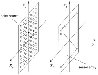
Assuming that equivalent sources are set on the acoustic source surface, represent the equivalent source intensity. The acoustic pressure signal is collected by sensors on the array. According to the propagation law of sound wave in the free field, the acoustic pressure on the measured surface can be approximated as follows:
The represents the free space Green's function from the equivalent source to the acoustic array. Generally, it can be rewritten into the form of matrix:
where is the equivalent source intensity vector, and the elements in the matrix of represent the transfer function between the -th equivalent source and the -th element:
The is the wave number. For the solution of Eq. (2), obtaining the equivalent point source intensity is the key to the equivalent source method. However, in practical applications, in order to display the detailed information in the acoustic field more precisely, more equivalent point sources will be set up to improve the resolution, and the number of array sensors is expected to be as small as possible, that is . This leads to the underdetermined problem of Eq. (2), whose solution subspace is not unique and needs to find its optimal solution.
The optimal solution of this problem is usually obtained by regularization. The traditional solution is to use Tikhonov regularization method to deal with, through the -norm of the solution vector to constraint, obtain the smooth minimum energy solution, and transform the solution of the equation into the minimization problem of the following function:
The acoustic pressure values obtained by this regularization method are consistent at the measurement points, but generally smaller at other locations. In the actual environment, the location of the acoustic source in space is sparse, and most of the values of equivalent source intensity vector are zero. Therefore, it is considered to obtain the optimal solution with the goal of sparseness, that is, to replace -norm with -norm to optimize the solution of Eq. (2):
For Eq. (5), this is a non-convex optimization problem, which is generally difficult to solve. According to the relevant theories of compressed sensing, this problem can be extended to the solution of Eq. (6) under certain conditions, that is, it can be converted into a -norm optimization problem. For the -norm optimization problem, convex optimization algorithm can be used to solve the problem. The specific algorithms include base tracking algorithm or gradient shadow algorithm:
By calculating the intensity of equivalent source, the acoustic quantity at any position in space can be calculated by acoustic transfer function, and the acoustic field reconstruction can be realized.
2.2. Measurement of incoherence of the sensing matrix
If the solution result of Eq. (6) is consistent with the solution of Eq. (5), Restricted Isometry Property (RIP) and Mutual Incoherence Property (MIP) [15] should be satisfied, which are two different expressions to measure the uncorrelation of the sensing matrix.
Under the theoretical framework of compressed sensing, only the sensor matrix with unrelated columns can ensure the recovery of sparse signals, and the matrix in Eq. (2) is the sensor matrix. The MIP condition is that any two different column vectors in the requirement are not correlated, which is generally expressed by the coherence coefficient and calculated according to Eq. (7):
where , represents any column vector in the matrix , represents the inner product. The smaller means the stronger incoherence of , which is more conducive to accurately calculating the intensity of the equivalent sound source.
Unlike the MIP, which only considers the correlation of several pairs of column vectors, the RIP contains S-element column vectors, which is more suitable for the evaluation of matrix irrelevance. The represents the sparsity of the solution vector. It can be calculated from the following inequality:
The sensor matrix is substituted into Eq. (8) to obtain the minimum value of . The is any S-sparse vector. The minimum value of is also known as the Restricted Isometry Constant (RIC), which can be used to measure the uncorrelation of the matrix .
For Eq. (8), the ideal is that when is a unitary matrix, at this time , is zero. It also shows that the matrix is completely column independent. However, due to the fact that calculated from the actual constructed sensing matrix is greater than zero.
In practical, because of the large dimension of sparse vector, it is very time-consuming to accurately solve the value of , which is difficult to achieve in reality. P. Simard [16] used Monte Carlo method and probability knowledge to find the statistical solution of , so as to quickly compare the uncorrelation degree of array sensing matrix.
Monte Carlo method is a kind of stochastic simulation calculation method, which can obtain the statistical parameters of the problem by random sampling without complicated formula calculation, so as to infer the approximate value of the parameters. First, the Eq. (8) is transformed into the form of Eq. (9), and then the sparse vector is randomly generated, which is substituted into Eq. (9) and solved. The statistical value of is obtained to the frequency histogram, as shown in Fig. 2, which is approximately Gaussian distribution:
Fig. 2Statistical histogram of δ
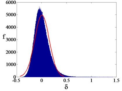
According to the statistical knowledge, the statistical values is in the interval [, ] with high probability. is the average and is the standard deviation. Therefore, the can be expressed through this interval, as shown in Eq. (10):
Therefore, the statistical estimation can represent the property of measurement matrix to a certain extent, and provide a certain basis for the solution of acoustic source.
3. Optimization of array design
The performance of the array has a great influence on the acoustic imaging effect. The work of array design mainly includes the determination of the number of sensors, the arrangement of array elements and the size of the array. The number of sensors determines the amount of information collected. The more information there is, the higher the accuracy of acoustic field reconstruction will be. However, a large number of sensors will increase the complexity and high cost of information processing. Therefore, in order to give full play to the signal acquisition capability of the array, a suitable arrangement method of acoustic array is sought through simulation under the condition of certain quantity and size.
For the sparse regularization of the acoustic source localization algorithm, random array is an ideal configuration (such as Gaussian random matrices). The traditional regular arrangement often has a certain spatial position correlation, which will lead to redundant and waste of the data collected by sensors, and unable to give full play to the role of the collected data. However, the specific random array design will be limited by the actual installation and measurement calibration level, which is difficult to realize in hardware. Therefore, pseudo-random arrangement is adopted in this paper to design the arrangement mode of array in a certain degree of dense grid.
The 1 m×1 m rectangle is uniformly divided into 20×20 grids to form 21×21 intersection points. Firstly, the array arrangement of 40 arrays is studied. By randomly selecting the positions of 40 intersection points as the placement points of the sensors, the minimum interval is 0.05 m, as shown in Fig. 3, and a pseudo-random array consisting of 40 arrays is obtained.
Fig. 3Pseudo-random array arrangement of 40 arrays
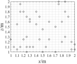
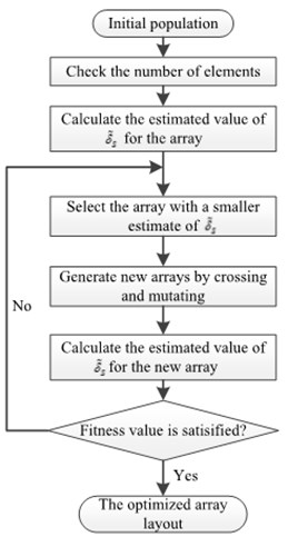
Fig. 4Algorithm flow
For arbitrary pseudo-random array arrangement, it is not possible to directly determine the pros and cons of performance, and because of the numerous arrangement methods, it is also impossible to rely on acoustic imaging algorithm to compare and test one by one.
Genetic algorithm can effectively solve the problem of nonlinear searching global optimal target. This algorithm selects the optimal solution by imitating natural selection, crossover and mutation. The array sensor positions are encoded as chromosomes, and crossover and mutation calculations are carried out, and is used as fitness value for screening. The calculation process is shown in Fig. 4.
4. Simulation experiment
4.1. Array parameters
In order to study the influence of array arrangement on acoustic imaging results, the array size and array element number should be set in a consistent manner. The array size is set as 1 m×1 m, and the number of array elements is controlled at about 40. The cross array and network array are arranged according to the regular, and the optimized pseudo-random array is obtained by iterative screening of genetic algorithm. The layout diagram of the cross array, network array and optimized pseudo-random array are shown in Fig. 5. The programmed algorithm is used to process the sound pressure values of the sound field collected by these arrays respectively, and the acoustic imaging effects of these arrays are compared.
Fig. 5Array layout data
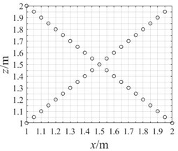
a) Cross array of 41 arrays

b) Grid array of 36 arrays
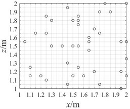
c) Optimize pseudo-random array of 40 arrays
4.2. Establishment of simulation model
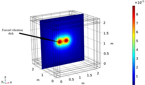
The modeling and simulation work is completed by the acoustics software COMSOL Multiphysics, and the pressure acoustics module is invoked, the double-disk interference sound field model is shown in Fig. 6. The first step in the modeling is to construct a cubic air domain with 2 m sides and add a perfectly matched layer (PML) with a thickness of 0.2 m to its exterior. The second step is to place two disks with a radius of 0.05 m and a thickness of 0.01 m as sound sources, and the center distance between them is 0.4 m. The materials are set as structural steel, and the edges of the disks are fixed and constrained. And a force of 50 N is applied to the center of these disks to excite the sound field. The third step is to place the data acquisition array, which is 0.2 m away from these disks, to collect the sound pressure data in the sound field. After modeling, free tetrahedral grids are used to divide the entire study area, and the division is conducted according to the rule of no less than 5 grids in one wavelength. The research object is the frequency of sound sources. In the frequency range of 50-2000 Hz, the sound field generated by the force exerted on disks is simulated and calculated with the step size of 50 Hz.
According to the Monte Carlo method mentioned above, the estimated values of of different arrays are calculated, and the preliminary comparison of different arrays is made. The results are shown in Table 1.
Table 1The estimates of δ~S for different arrays
The array distribution | Cross array | Grid array | Optimize pseudo-random array |
0.4383 | 0.4723 | 0.4026 |
From the numerical of point of view, the optimal pseudo-random array is the most suitable array for the acoustic holography algorithm, which satisfies the limit of 0.4625 proposed by Foucault, and meets the requirements of the RIP conditions.
Fig. 6Excitation sound field model of double disk
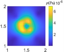
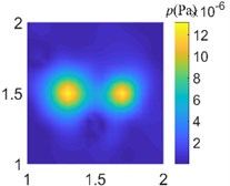
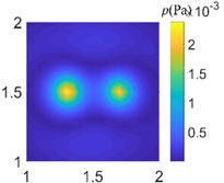
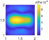
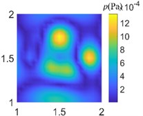
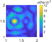
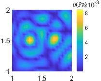
In order to compare the acoustic imaging effect of different arrays, the data collected from different arrays are used for acoustic field reconstruction. After processing by sparse regularization equivalent source algorithm, the acoustic images of different arrays are compared. As shown in Fig. 7-9, the acoustic pressure distribution at a distance of 0.1 m from the sound source is reconstructed at 50 Hz, 500 Hz, and 1000 Hz respectively. It can be clearly seen from the figure that the data collected by regular traditional array cannot accurately reconstruct the acoustic field acoustic pressure through the algorithm under different frequencies, which will misjudge the location and quantity of acoustic sources and cannot guide the location of acoustic sources; The data collected by the optimal pseudo-random array are processed by the same algorithm to get the acoustic pressure distribution closer to the actual acoustic field, which is in line with the actual acoustic pressure distribution on the whole, and shows the acoustic source location accurately without missing or misjudgment.
Fig. 7Acoustic pressure reconstruction of different arrays (f= 50 Hz)
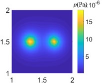
a) Ideal measured value
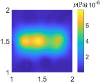
b) Grid array of 36 arrays
c) Cross array of 41 arrays
d) Optimize pseudo-random array of 40 arrays
Fig. 8Acoustic pressure reconstruction of different arrays (f= 500 Hz)
a) Ideal measured value
b) Grid array of 36 arrays
c) Cross array of 41 arrays
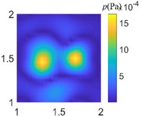
d) Optimize pseudo-random array of 40 arrays
Fig. 9Acoustic pressure reconstruction of different arrays (f= 1000 Hz)
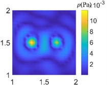
a) Ideal measured value
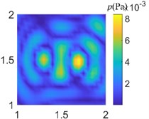
b) Grid array of 36 arrays
c) Cross array of 41 arrays
d) Optimize pseudo-random array of 40 arrays
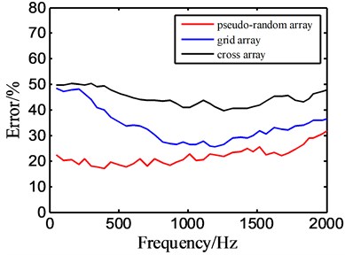
In order to accurately describe the difference between the reconstructed acoustic pressure and the actual situation, the reconstruction error is generally calculated by Eq. (11):
where is the reconstructed acoustic pressure value matrix at 0.1 m away from the acoustic source, and represents the actual acoustic pressure value matrix at 0.1 m away from the acoustic source in the simulation environment. The reconstruction errors corresponding to different arrays are calculated, and Fig. 10 is drawn. The figure shows the variation of reconstruction error from low frequency to high frequency for different arrays.
It can be seen from the Fig. 10 that the reconstruction errors of cross array and grid array are larger, and the errors under different frequencies are quite different. The reconstruction error of the optimized pseudo-random array is smaller than that of the other two arrays, and it has a good reconstruction effect in a wide frequency range, which can be used to indicate the position of acoustic source.
Fig. 10Reconstruction error graph
5. Conclusions
The imaging principle of the equivalent source acoustic holography algorithm is analyzed, and the effect of array layout on the imaging effect is analyzed from the perspective of the sensor matrix irrelevance in this paper. For sparse regularized equivalent source holographic algorithms, the more irrelevant the sensor matrix is, the better the accuracy of acoustic field reconstruction will be. Moreover, such irrelevance can be measured by the Restricted Isometry Constant. According to this characteristic, by using the advantage of intelligent algorithm to solve the global optimal value, the optimal pseudo-random array arrangement of 40 array elements is selected. By comparing the acoustic imaging effect of traditional regular array, the optimized array has obvious advantages and can be used in the design of acoustic array system.
References
-
Chunlei Li, Qiang Han, Zhan Wang, et al. Analysis of wave propagation in functionally graded piezoelectric composite plates reinforced with graphene platelets. Applied Mathematical Modelling, Vol. 81, 2020, p. 487-505.
-
Haibin Yang, Yong Xiao, Honggang Zhao, et al. On wave propagation and attenuation properties of underwater acoustic screens consisting of periodically perforated rubber layers with metal plates. Journal of Sound and Vibration, Vol. 444, 2019, p. 21-34.
-
Ayse Nihan Basmaci Characteristics of electromagnetic wave propagation in a segmented photonic waveguide. Journal of Optoelectronics and Advanced Materials, Vol. 22, Issues 9-10, 2020, p. 452-460.
-
Eldad Jitzchak Avital, Neeshtha Devi Bholah, Giuseppe Cortez Giovanelli, et al. Sound scattering by an elastic spherical shell and its cancellation using a multi-pole approach. Archives of Acoustics, Vol. 42, Issue 4, 2017, p. 697-705.
-
Luo Ziren, Zhang Min, Jin Gang Comprehensive discussion on the core problems of laser interferometric gravitational wave space array. Chinese Science Bulletin, Vol. 64, Issue 24, 2019, p. 2468-2474, (in Chinese).
-
Pan Changchang, Baronio Fabio, Chen Shihua Research progress of extreme wave events in integrable resonant systems. Journal of Physics, Vol. 69, Issue 1, 2020, p. 49-60, (in Chinese).
-
Valdivia N. P. Advanced equivalent source methodologies for near-field acoustic holography. Journal of Sound and Vibration, Vol. 438, 2019, p. 66-82.
-
Chu Zhigang, Ping Guoli, Yang Yang, et al. Determination of regularization parameters in near-field acoustical holography based on equivalent source method. Journal of Vibroengineering, Vol. 17, Issue 5, 2015, p. 2302-2313.
-
Hu DingYu, Li Hebing, Hu Yu, et al. Sound field reconstruction with sparse sampling and the equivalent source method. Mechanical Systems and Signal Processing, Vol. 108, 2018, p. 317-325.
-
Zhao Yongfeng, Yang Tao Near-field acoustic holography based on compressive sensing by using the smoothed l0 norm method. Piezoelectrics and Acoustooptics, Vol. 40, Issue 1, 2018, p. 73-78, (in Chinese).
-
Elad M. Sparse and Redundant Representations: From Theory to Applications in Signal and Image Processing. Springer, New York, 2010.
-
Yang Yang, Cai Pengfei, Chu Zhigang The influence of array geometry and element failure on SONAH reconstruction results. Technical Acoustics, Vol. 4, 2014, p. 352-358, (in Chinese).
-
Jorgen Hald Combined NAH and beamforming using the same microphone array. Sound and Vibration, Vol. 38, Issue 12, 2004, p. 18-27.
-
Chardon G., Daudet L., Peillot A., et al. Near-field acoustic holography using sparse regularization and compressive sampling principles. The Journal of the Acoustical Society of America, Vol. 132, Issue 3, 2012, p. 1521-1534.
-
Donoho D. L., Huo X. Uncertainty principles and ideal atomic decomposition. IEEE Transactions on Information Theory, Vol. 47, Issue 7, 2001, p. 2845-2862.
-
Simard P., Antoni J. Acoustic source identification: Experimenting the L1 minimization approach. Applied Acoustics, Vol. 74, Issue 7, 2013, p. 974-986.
About this article

