Abstract
Inlet flow distribution devices play an important role in providing uniform flow distribution in water treatment process units such as sedimentation tanks. Orifices and weirs are commonly provided along the inlet flow channels that are built across the width of sedimentation tanks. This paper presents a numerical method and computer program for computation of the inlet flow distribution over weirs and orifices. The method is based on solving a differential equation of the flow profile along the flow distribution channel using numerical technique, namely, the Runge-Kutta method. The method replaces the trial and error step employed in earlier methods in the determination of weir discharge depths. Application examples are provided in which more uniform flow distribution were achieved by employing wider channel and full tapering of the inlet flow channel geometry or through partial tapering of the ends of the channel. The method can be extended for computation of inlet flow distribution in other similar water and wastewater treatment process units that employ weirs and orifices.
Highlights
- A numerical method for analysing inlet flow distribution to sedimentation tanks has been developed
- A differential equation for analysing inlet flow distribution has been solved using the Runge Kutta method
- A computer programme has been written to solve the differential equation numerically
- Various inlet flow profiles have been analysed to examine their influence on flow distribution
- The method can be adapted for inlet flow systems that accurately model the discharge coefficient variation
- The method fits into semi empirical approaches for solving inlet flow distribution problems
1. Introduction
Uniform flow distribution across process units in water and wastewater treatment is necessary to assure proper operation and performance of the units. In water treatment, non-uniform flow in sedimentation tanks can result in turbulence, dead zones and short circuiting that cause deviation of the solids settlement from the designed conditions. Flocculation units must receive flows distributed equally among the same units failing which those units with shorter retention time can experience floc break up and floatation of sludge [1]. An unusually long retention time in wastewater treatment units because of non-uniform flow distribution can result in large sludge age and sludge decay [2].
Inlet flow distribution devices such as weirs and orifices at inlet flow channels or baffle walls placed across the width of sedimentation assist in distributing flows uniformly over the flow space and increasing the detention time as well as minimizing short circuiting. Perforated baffle walls play a big role in modifying the flow regime and equalizing flows within sedimentation tanks [1, 3]. The method developed by Chao and Trussel [4] is commonly used for analysing inlet flow distribution among weirs and orifices provided along the flow distribution channel. It is a one dimensional energy equation coupled with weir flow equation that involves a trial and error procedure for determining the flow profile across the weir. In order to overcome the non-uniform flow among the flow distribution weirs modifications have been proposed such as tapering the channel along the flow, varying the weir elevation among the different weirs, or using a combination of these modifications [5]. Ramamurthy [6] proposed a combination of weir and orifices (called weir-orifice units) acting in unison to equalise the variable flows in wastewater treatment process units that may vary during the different times of the day.
However, the use of complicated flow control devices within inlet flow channels that significantly modify the flow regime cannot be analysed accurately with simple one or two dimensional models. A simplified design such as using the [4] step method gave rise to errors because of unsatisfactory representation of the inlet flow due to abrupt change in flow direction. Practical observation showed that water treatment efficiencies were impaired as a result [7, 8]. A more accurate three dimensional analysis such as using computational fluid dynamics (CFD) modelling would be able to handle complicated flow distribution geometry [2].
Nowadays CFD models are available to study the effect of inlet flow distribution devices on the hydrodynamic behaviour and movement of water within reactor tanks. Such models are also supported by actual measurement of velocity at points within the reactor tank using acoustic Doppler velocimetery [1]. Computational fluid dynamic (CFD) models typically use finite volume analysis by splitting the volume of the reactor tank into large number of small grid volumes (cells) within which the fluid momentum and continuity equations are formulated together with specification of the boundary conditions for different flow conditions [9-11].
The effect of uniform flow distribution devices using more refined CFD models has been studied by a number of researchers and significant improvement in agreement between the model and reality has been reported [1, 12-16]. Park et al. [3] proposed providing diffuser walls inside flow distribution channel to achieve a more uniform flow distribution. Lee et al. [17] reported up to 30 % improvement in flow distribution through the use of a longitudinal baffle with orifices in the main flow direction. The effect of the longitudinal perforated baffle is to create a frictional flow resistance against unequal lateral flow towards the flow distribution orifices. The water level would equalise along the longitudinal channel length and this uniform water level assists in more uniform distribution of flow across the orifices or weirs provided. Knatz et al. [18] suggested gateway and mixing zone for improving flow distribution.
1.1. Semi empirical approach to flow distribution modelling
Despite the drawbacks observed in earlier models in accurately describing the flow behaviour along inlet flow distribution channels, semi empirical methods, if accurately modelled, still offer an opportunity for simpler and easy to use approximation to flow distribution. A better empirical relationship between discharge coefficient and velocity distribution in the longitudinal and transverse direction with respect to the length of the channel can be obtained through experimental modelling to establish such relationship. The variation of the coefficient of discharge with the upstream Froude Number is indicated through dimensional analysis which indicates the coefficient of discharge is a function of the upstream Froude Number and the ratios of length of the channel to the width, length of the channel to water depth and the ratio of the crest height to the water depth [19].
Rao and Pillai [20] experimentally studied the spill component of the velocity along the channel direction, i.e., the component of the velocity in the direction of the channel length of the water that is flowing over the weir. This is a component that is neglected in the earlier methods for example developed by Chao and Trussel [4] which led to the significant deviations of the modelled output of flow distribution from what was actually observed in the real case. According to the result of Rao and Pillai [20], the ratio of the upstream channel length velocity to the spill component of the velocity in the same direction / is related to the upstream Froude Number by a convex shaped parabolic equation obtained through regression of the experimental data. In addition, the variation of the discharge coefficient with the upstream Froude Number is modelled through a parabolic relationship obtained from experimental data. Rather than using the energy equation alone, the use of the momentum equation along the channel length enables the incorporation of the spill component of the flow velocity along the channel length. The resulting flow profile along the channel has better accuracy compared to the earlier methods. However, the results still can be improved further if other variables indicated by dimensional analysis are taken into account, namely, the ratios of length of the channel to the width, length of the channel to water depth and the ratio of the crest height to the water depth.
According to the research experiment carried out by Mohammed [21], the discharge coefficient could be related not only to the upstream Froude Number but also to the ration of the channel dimensions as well as the upstream depth of flow as indicated by dimensional analysis. The resulting equation for discharge coefficient is a multi linear function of the non-dimensional variables, namely the upstream Froude number, the ratio of the weir crest height to depth as well as the ratio of the channel length to depth. This equation seems consistent with much higher coefficient of regression ( 0.95) compared with the results obtained by earlier researchers. The resulting model is also more accurate as verified by comparison with model output carried out by detailed computational fluid mechanics methods. The results also agree closely with experimental measurements while Euler’s method is applied for computing the water depth profile as well as the discharge.
The effect of the upstream Froude Number of the discharge coefficient was also studied by Mahmodiniaa et al [22) using the FLUENT hydraulic computation software. The result revealed the dependence of the discharge coefficient on the upstream Froude Number. A more accurate model based the dimensional analysis results was obtained by Azza [23] in which the discharge coefficient for side weirs at different oblique angles was related to the non-dimensional parameters using power equations with the model results agreeing closely with experimental observations. Swamee et al [24] also found pout the discharge coefficient varying with the water depth to weir height ratio for skew weirs. Samani [25] also shows the dependence of the discharge coefficient with the channel length to width ratio in the form of a cubic equation. Oertel et al [26] also showed the dependence of flow and discharge coefficient on the geometric characteristics of the channel. Di Bacco and Scorzini [27] also emphasized the need to take into account the effect of consistent set of relevant parameters such as the friction factor in determination of discharge coefficients. Borghei et al [28] also suggested the sensitive parameters that influence the discharge coefficient to be the upstream Froude Number, the ratio of the crest height to depth of water and the ratio of channel length to channel width.
2. Methodology
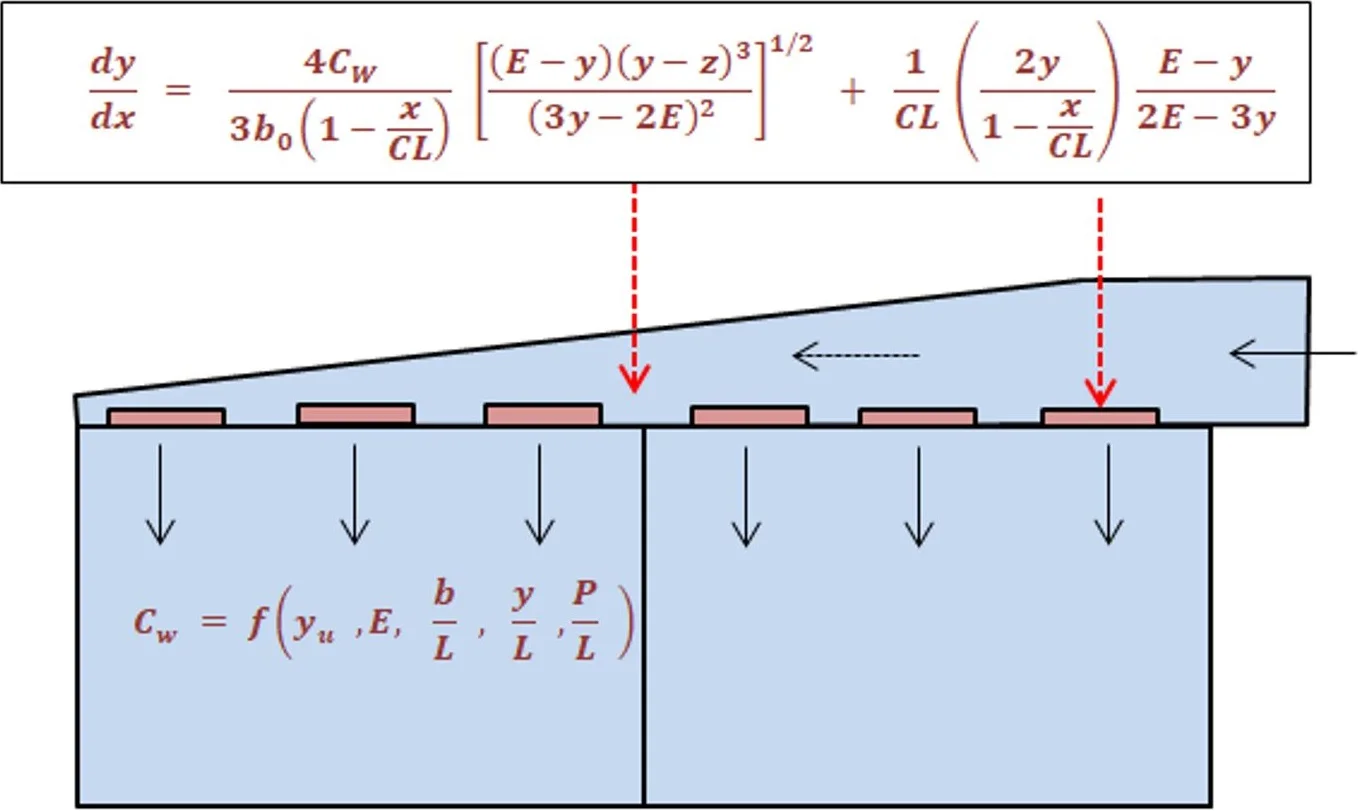
The method of flow distribution analysis presented in this paper is a modification of the step method proposed by Chao and Trussel (1980) by eliminating the trial and error procedure for determining the flow profile between the weirs and replacing it with a differential equation of the flow profile that is solved using the Runge-Kutta method. The method will enable analysis of flow distribution as well as optimization of the flow distribution in simple geometry of the channels. The derivation of the equation needed to distribute flows along weirs of common fed channels will be presented below. The equation applies to orifices as well except that the discharge equation has to be modified accordingly. Considering a uniformly tapered channel of initial width , shown in Fig. 1, the width of the channel at a distance from the inlet end is:
Fig. 1Plan view of the inlet flow distribution channel with tapered geometry
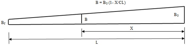
The value of in Eq. (1) varies from 1 for 0 to for . Assuming a constant specific energy along the channel length by neglecting frictional loss over small length of the channel, the discharge can be expressed in terms of the constant specific energy as follows:
Solving the above equation for the discharge , one gets:
The equation of discharge q over a sharp crested weir of width is given by:
In Eq. (3) is the discharge coefficient, is the weir length, is the weir elevation measured from the bottom of the channel and is the depth of water in the channel. The rate of change of flow over the channel length as the flow passes through the weir section is then given by:
The same rate of change of flow with distance along the channel given in Eq. (4) can also be calculated by differentiating in Eq. (2) with respect to as follows:
Since the width b of the inlet flow distribution channel is variable along the channel length as given by Eq. (1), the term in Eq. (5) is computed from Eq. (1) as:
Substituting the expression for given by Eq. (6) in Eq. (5) one gets:
Equating Eq. (4) and Eq. (7), i.e.:
Solving for :
Substituting the expression for b in Eq. (1) into Eq. (8) and simplifying further gives:
Eq. (9) is a first order differential equation in and can be readily solved using numerical techniques. In this particular case the Runge-Kutta method has been chosen to solve the differential equation for the depth of flow y over the channel length. A computer program using the BASIC language has been implemented in order to carry out the discharge computation over each weir based on the differential equation given by Eq. (9).
For the channel section along which there is no weir flow, setting 0 in Eq. (9) gives:
Over the channel section where there is weir flow, the coefficient of discharge varies with the upstream Froude number and is given by:
In Eq. (11) is the Froude number of the channel flow just upstream of the weir and is the upstream channel flow depth. is the specific energy of flow in the channel as defined earlier. The depths at each section are determined by numerical integration of Eq. (9) or Eq. (10) using the Runge-Kutta formula. Once the depths are determined at upstream and downstream of the weir, the average depth is used to calculate the flow over the weir.
3. Results and discussion
The derivation of the equation given by Eqs. (9), (10) and (11) allows computation of the weir discharges using numerical methods by applying the Runge-Kutta method. In order to implement the computation using a BASIC computer program, a procedure and flow chart has been prepared which is outlined below. The implementation of the computer program is carried out using an example of inlet flow distribution of sedimentation basins of a water treatment plant as will be described in detail later.
The following procedure is employed in the computation of discharge over each weir:
Step 1. Initialize the discharge through the first weir by uniformly distributing the total discharge between the weirs:
where is the discharge through the first weir and is the number of flow distribution weirs over the channel.
Step 2. Initialize the discharge coefficient for the first weir as 0.611 and compute the average depth over the first weir of length using Eq. (3):
Step 3. Now it is possible to start with as the upstream depth . Calculate the channel velocity upstream of the first weir and the channel flow specific energy:
Step 4. Revise the upstream discharge coefficient with the specific energy calculated in step 3 using Eq. (11):
Step 5. Compute the depth downstream of weir number 1, i.e., by successive numerical integration of the differential equation given by Eq. (9) using the Runge-Kutta method. Afterwards, revise the average depth of flow over weir 1 as:
Step 6. Revise the computation of the discharge over the first weir using Eq. (3):
Step 7. Moving along the channel for which there is no weir flow, determine the channel flow depth upstream of the second weir, , by numerical integration using Runge-Kutta method of the differential equation given by Eq. (10).
Step 8. Compute the discharge coefficient for the second weir in the manner of step 4, i.e.:
Step 9. Compute the average flow depth over the second weir and the discharge over the same year using respectively the formulae given in step 5 and step 6.
Step 10. Repeat the computation of flow over the remaining weirs similarly following the steps given above.
Step 11. Calculate the total sum of discharge over the weirs:
Step 12. Calculate the error in the computation of the total discharge over the channel:
If is less than a prescribed allowable error in the computation of discharges, say for example, 0.001, the discharge computation is accurate enough and no further computation is necessary. If not proceed to step 13.
Step 13. Distribute the correction to the discharge over the first weir in proportion to its value as follows:
Step 14. From the weir flow formula given in Eq. (3), i.e.:
Calculate the incremental depth using the differential relation between and . This relation is given as:
Step 15. Compute the revised upstream depth of the first weir for the second iteration as:
Step 16. Now go back to step 3 and repeat the whole process until the discharge distribution over the weirs sums to the total discharge within the specified accuracy.
The flow chart is given in Fig. 2. It is noted that the procedure above eliminates the trial and error procedure at each weir length which was necessary in the former method developed by Trussel, et al (1980). An example from (Trussel, et al., 1980) is reproduced again here and the problem is solved using the procedures described above.
3.1. Example problem
A water treatment plant is to handle a flow of 15 mgd (56800) m3/day. The flow enters from one end of the influent channel and distributes it to sedimentation basins through six side weirs. The channel is 14.63 m long and 1.219 m wide. The side weirs are 1.21 m wide and placed 1.21 m apart (Fig. 3-5). Estimate the discharge distribution through the weirs.
Solution:
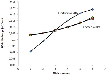
The flow distribution has been analysed using the computer program developed and presented here. The results are shown in in Table 1 and Table 2 It is noted that there is a 30 % difference in the flows between the upstream and downstream weirs when a uniform channel width of 1.2 m is used. This flow distribution is non-uniform and inadequate. The flow towards the end weirs is greater than those at the front. This is shown clearly in Fig. 6 in which the flows over the different weirs vary markedly from the minimum at the inlet to the flow distribution channel to the maximum at the end of the channel.
In order to overcome this non-uniform flow distribution over the weirs, the program was run by assuming a wider channel width at the top ( 1.8 m) and full tapering in which the width at the end of the flow distribution channel is zero. The resulting discharge over the weirs shown in Table 1 and Table 2 is a marked improvement. The difference between the maximum and minimum discharges is reduced from 30 % to about 11 %.
Similar level of equalization was achieved by assuming a uniform wide channel section for the first four weirs and full tapering carried out only after the fourth weir, i.e., the last 5.5 m length of the flow distribution channel. The resulting flow distribution shown in Table 1 and table 2 is a gain a marked improvement in which the difference between the minimum and maximum weir discharges is reduced from 30 % of the average flow to about 12 %.
Fig. 2Flow chart of the BASIC program for computation of inlet flow distribution over weirs
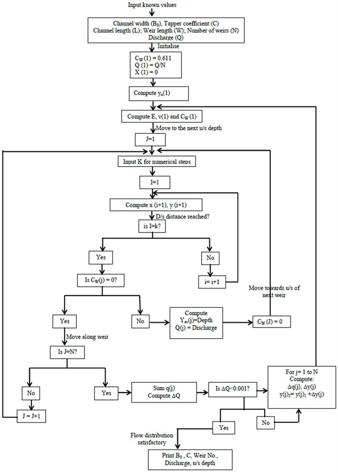
Fig. 3Vertical x-sectional view of the sedimentation basins
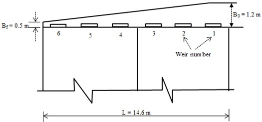
Table 1Result of the BASIC program of inlet flow distribution computation
Weir number | Uniform channel width ( 1.2 m) | Wide channel with full tapering (1.8 m) | Wide channel with tapering after the 4th weir ( 1.8 m) | |||
US depth (m) | Discharge (m3/sec) | US depth (m) | Discharge (m3/sec) | US depth (m) | Discharge (m3/sec) | |
1 | 0,7300736 | 0,09088982 | 0,7412963 | 0,1039732 | 0,7425668 | 0,1037204 |
2 | 0,7376601 | 0,09883455 | 0,7423991 | 0,1054316 | 0,7438427 | 0,1052179 |
3 | 0,7443541 | 0,1076434 | 0,743799 | 0,1075193 | 0,7454051 | 0,107364 |
4 | 0,749992 | 0,1151424 | 0,7456051 | 0,1101727 | 0,7473234 | 0,1100075 |
5 | 0,7542778 | 0,1207819 | 0,7479282 | 0,1134506 | 0,7496372 | 0,1132149 |
6 | 0,7569484 | 0,1241081 | 0,7507537 | 0,1168527 | 0,7518371 | 0,1178753 |
Table 2Variation of discharge flows among the different weirs
Uniform channel width ( 1.2 m) | Wide channel with full tapering ( 1.8 m) | Wide channel with tapering after the 4th weir (1.8 m) | |
Mean discharge | 0,109566695 | 0,109566683 | 0,109566667 |
Standard deviation | 0,012930781 | 0,004921704 | 0,00530056 |
Coefficient of variation | 11,80 % | 4,49 % | 4,84 % |
Maximum discharge | 0,1241081 | 0,1168527 | 0,1178753 |
Minimum discharge | 0,09088982 | 0,1039732 | 0,1037204 |
Range | 0,03321828 | 0,0128795 | 0,0141549 |
Range (%) | 30,32 % | 11,75 % | 12,92 % |
Fig. 4Inlet flow distribution weir profile
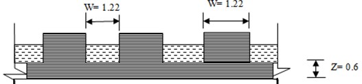
Fig. 5Plan of the tapered geometry of the inlet flow distribution channel
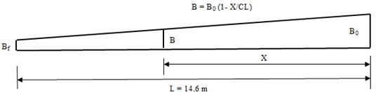
Fig. 6Variation of discharge over the different flow distribution weirs
4. Discussion
The use of semi empirical approach to the modeling of flow distribution over weirs provided along the inlet channels such as sedimentation can be a useful simplified approach that will provide reasonably accurate results if modeled properly. The equations and computer program developed were used for modeling the water depth and discharge by solving the differential equation using the Runge- Kutta method. Different channel shapes and dimensions can be tried in order to provide the optimum flow distribution over the weirs along the channel. As demonstrated through the examples, tapering the channel width resulted in a more uniform flow distribution. Likewise other parameters such as height of weir crest can also be varied in a similar to arrive at the optimal solution. Accurate modeling of the water surface profile is possible along the weir flow since the differential equation can be solved using smaller step.
The drawback of using the average height for calculating the discharge coefficient can be overcome by a more accurate experimental modeling as is mentioned in the introduction section. Once the discharge coefficient is accurately modeled using the relation between the discharge coefficient and relevant parameters such as upstream m Froude number, ratio of weir height to water depth and ratio of channel length to channel width. The developed equation and program shown in this paper can be easily adapted to solve for the flow distribution. In addition, the influence of the spill component of the velocity in the channel length direction can also be taken into account and the momentum approach shown by Rao and Pillai [20] can also be used as basis for the approach developed in this paper to solve for the flow distribution over the weirs. The semi empirical approach can be further expanded by taking in to account other variables such as friction factor and channel slope. Where there are too many variables making classical regression difficult. Neural network approaches can be carried out to determine the discharge coefficient as a function of several relevant variables through a model developed using neural networks. This has been demonstrated by Ayaz and Mansoor [29].
The drawback of earlier semi empirical models to flow distribution over weirs along inlet channels can, therefore, be reduced and the accuracy improved through experimentally determined relationship between the discharge coefficient and the non-dimensional parameters as indicated by dimensional analysis using Buckingham Pi theorem. In addition, the use of momentum approach and considering energy loss, friction factor as well as channel slope will add to the accuracy of the analysis results.
5. Conclusions
The performance of water treatment units such as sedimentation tanks is strongly influenced by the manner in which flow is distributed in the reactor tanks. In order to maximise the detention time of solids in sedimentation tanks and minimise turbulence, dead end zones and short circuiting, providing uniform flow distribution devices at the inlet of sedimentation tanks is helpful. Weirs and orifices are often provided at inlet to sedimentation tanks as uniform flow distribution devices.
A numerical method for determining flow distribution among weirs and orifices at inlets to sedimentation tanks is presented. The procedure is based on solving a differential equation of the channel water depth with respect to the channel length by numerical techniques applying the Runge-Kutta method. The method so developed eliminates the trial and error procedure for determining depths in calculating the flows over the individual weirs. Application of the method has been demonstrated using an example of flow distribution over weirs provided at inlet channels of sedimentation tanks. According to the results, a uniform channel width produced a variation in flow distribution among weirs as high as 30 % of the average flow. Using a wider channel coupled with full tapering in the form of a triangular geometry produced a more uniform flow distribution that reduced the variation between the maximum and minimum flows among the weirs to 11 % of the average flow. Further modification of geometry of the inlet flow channel by tapering only the last 40 % of the channel length also produced similar distribution flow among the weirs in which the variation between the maximum and minimum flows is about 12 %.
The method demonstrated can be applied further for optimisation of the geometry of the inlet flow distribution channel so that uniform flow distribution is achieved over the length of the inlet flow distribution channel. The computer program developed in the BASIC language has been summarised through the flow chart presented and is easy to implement in any other programming language. This method may also be adapted for computation of flow distribution in other types of channels than sedimentation tanks.
References
-
Baek H. K., Park N. S., Kim J. J., Lee S. J., Shin S. J. L. Examination of three-dimensional flow characteristics in the distribution channel to the flocculation basin using computational fluid dynamics simulation. Journal of Water Supply: Research and Technology, Vol. 54, Issue 6, 2005, p. 349-354.
-
Park N. S., Yoon S., Jeong W., Lee S. Improving flow distribution in influent channels using computational fluid dynamics. Water Science and Technology, Vol. 74, Issue 8, 2016, p. 1855-1866.
-
Park N. S., Kim S. S., Park J. Y., Yoon C. H., Kim C. H. The remodelling of hydraulic structure in a distribution channel for improving the equality of the flow distribution (I): design using CFD simulation. Journal of the Korean Society of Water and Wastewater, Vol. 21, Issue 5, 2007, p. 571-579.
-
Chao J. L., Trussel R. R. Hydraulic design of flow distribution channels. Journal of the Environmental Engineering Division of the American Society of Civil Engineers, Vol. 106, 1980, p. 321-333.
-
Benefield L. D., Judkin J. F., Parr A. D. Flow in Open Channels, Treatment Plant Hydraulics for Environmental Engineers. Prentice-Hall, New York, 1984, p. 108-122.
-
Ramamurthy A., Tim U., Rao M. Weir-orifice units for uniform flow distribution. Journal of Environmental Engineering, Vol. 113, Issue 1, 1987, p. 155-166.
-
Hudson E. H. Water Clarification Processes Practical Design and Evaluation. Van Nostrand Inc., New York, 1981, p. 258-275.
-
Baek H. K., Kim W. K. Rapid Mixing and Flocculation Basins, Composite Correction Program for Seoungnam Water Treatment Plant. Korea Water Resources Corporation, Deajon, 2000, p. 48-105.
-
Sicilian J. M., Hirt C. W., Harper R. P. FLOW-3D: Computational Modelling Power for Scientists and Engineers. Flow Science Report (FSI-87-00-1), Flow Science, 1987.
-
Park N. S., Park H., Kim J. S. Examining the effect of hydraulic turbulence in a rapid mixer on turbidity removal with CFD simulation and PIV analysis. Journal of Water Supply Research and Technology, Vol. 52, Issue 2, 2003, p. 95-108.
-
Hirt C. W., Nichols B. D. Volume of fluid (VOF) methods for the dynamics of free boundaries. Journal of Computational Physics, Vol. 39, 1981, p. 201-210.
-
Ta T. C. Current CFD tool for water and waste water treatment processes. Pressure Vessels and Piping Division (Publication) PVP, Vol. 396, 1999, p. 79-85.
-
Dutta S., Catano F., Liu X., Garcia M. Computational fluid dynamics (CFD) modelling of flow into the aerated grit chamber of the MWRD’s North Side Water Reclamation Plant, Illinois. Proceedings of the World Environmental and Water Resources Congress, 2010, p. 1239-1249.
-
Lin F. Improving Flow Distributions in Treatment Plants Using CFD Modelling. Stantec for Pacific Northwest Clean Water Association, 2012, http://www.pncwa.org/.
-
Nopens I., Batstone D., Griborio A., Samstag R., Wicklein E., Wicks J. Computational fluid dynamics (CFD): what is good CFD-modelling practice and what can be the added value of CFD models to WWTP modelling. Proceedings of WEFTEC, 2012.
-
Park N. S., Park H., Kim J. S. Examining the effect of hydraulic turbulence in a rapid mixer on turbidity removal with CFD simulation and PIV analysis. Journal Water Supply: Research & Technology – AQUA, Vol. 52, Issue 2, 2007, p. 95-108.
-
Lee A., Park N., Kim S., Kim N. Physical modifications to improve a channel’s flow distribution. Korean Journal of Chemical Engineering, Vol. 29, Issue 2, 2012, p. 201-208.
-
Knatz C., Rafferty S., Delescinskis A. Optimization of water treatment plant flow distribution with CFD modelling of an influent channel. Water Quality Research Journal of Canada, Vol. 50, Issue 1, 2015, p. 72-82.
-
Chow V. T. Open Channel Hydraulics. McGraw-Hill, New York, 1959, p. 439-460.
-
Rao K. H. V. D., Pillai C. R. S. Study of flow over side weirs under supercritical conditions Water Resources Management, Vol. 22, 2008, p. 131-143.
-
Mohammed A. Y. Numerical analysis of flow over side weir. Journal of King Saud University – Engineering Sciences, Vol. 27, 2015, p. 37-42.
-
Mahmodiniaa S., Javanb M., Eghbalzadehb A. The effects of the upstream Froude number on the free surface flow over the side weirs International Conference on Modern Hydraulic Engineering, Procedia Engineering, Vol. 28, Issue 1, 2012, p. 644-647.
-
Azza N., Al Talib Flow over oblique side weir. Damascus University Journal, Vol. 28, Issue 1, 2012, p. 15-22.
-
Swamee P., Ojha C., Mansoor T. Discharge characteristics of Skew Weirs. Journal of Hydraulic Research, Vol. 49, Issue 6, 2011, p. 818-820.
-
Samani K. Analytical approach for flow over an oblique weir. Journal of the Transaction of the American Society of civil Engineering, Vol. 17, Issue 2, 2010, p. 107-117.
-
Oertel M., Carvalho R. F., Janssen R. Flow over a rectangular side weir in an open channel and resulting discharge coefficients. 34th International Association of Hydraulic Research, Brisbane, Australia, 2011.
-
Di Bacco M., Scorzini A. R. Are we correctly using discharge coefficients for side weirs? Insights from a numerical investigation. Water, Vol. 11, 2019, p. 2585.
-
Borghei Jalili S. M. M. R., Ghodsian M. Discharge coefficient for sharp-crested side weir in subcritical flow. Journal of Hydraulic Engineering, Vol. 125, Issue 10, 1999, p. 1051-1056.
-
Ayaz M. D., Mansoor T. Discharge coefficient of oblique sharp crested weir for free and submerged flow using trained ANN model. Water Science, Vol. 32, 2018, p. 192-212.
About this article

