Abstract
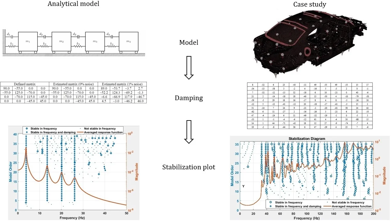
A verified computational model of a complex structure is crucial for reliable vibro-acoustic simulations. Mass and stiffness matrices of such a computational model may be constructed correctly, provided all the design information is available. Since it is an unknown, the damping matrix is usually populated through mathematical models based on some assumptions. In the current study, it is proposed to use the identified non-proportional structural damping matrix in the computational model. Structural damping matrix can be identified using the complex frequency response functions obtained from experimental modal analysis data. No matter what type of a damping mechanism a structure has; proportional or non-proportional, the frequency response functions of the system can be measured. First, the calculation procedure for the non-proportional structural damping matrix is explained. The damping matrix of an analytical model is identified successfully using the proposed procedure. The same procedure is then applied through a case study. Computational model of a test vehicle is constructed. Next, the test vehicle is subjected to a modal test to measure the frequency response functions of the structure. Incompleteness of the measured data and the requirements of the procedure are discussed, as well. The described procedure can be used in any model updating framework.
Highlights
- A non-proportionally damped analytical model is introduced
- The calculation procedure for the structural damping matrix is explained
- The same procedure is applied on a complex structure
- Incompleteness of the measured data and the requirements of the procedure are discussed
- The calculated stabilization plots of the analytical and complex models are given
1. Introduction
A multi degree of freedom (MDOF) structure is theoretically modelled in terms of mass, stiffness and damping matrices. One can assume that the mass matrix can be known correctly, but the stiffness matrix cannot [1]. To update a model, Baruch proposed to use an optimally corrected stiffness matrix. Berman and Nagy proposed to update both mass and stiffness matrices of a system using a method that minimizes the weighted norm of difference between analytical and measured structural modes subject to orthogonality constraints [2]. Wei offered to use the experimental modal model as a reference [3]. Friswell et al. proposed to update mass, stiffness and damping matrices simultaneously, using the measured modal data [4]. Carvalho et al. computed the unknown components of an experimental modal model [5]. Jacquelin et al. considered the uncertainties in the measurement results [6]. They offered a probabilistic method for model updating. These techniques [1-6] are known as direct methods. In direct methods, structural connectivity information cannot be preserved. Hence, to interpret the physical meaning of the results is a difficult task. Another drawback of this method is that the updated system matrices are not symmetric and positive definite.
Yet another approach used in the model updating studies is to improve the correlation of computational and experimental data by making iterations subject to modal parameters. These techniques are commonly known as iterative methods. Computations performed using iterative methods result in symmetric and positive definite system matrices. Lin and Ewins used the response function method (RFM), where the frequency response functions (FRFs) are employed for an iterative model updating [7]. Kwon and Lin made use of Taguchi method to optimize an objective function, which is determined up to the differences between computational and measured data [8]. Kim and Park proposed an automated parameter selection procedure for iterations [9]. Arora studied the prediction capabilities of an iterative model updating method, which also counts on damping matrices [10]. Mottershead et al. presented the guidelines of use of the sensitivity analysis in model updating [11]. Matta and Stefano investigated the modelling errors in their study that concerns the model updating of a large-scale building structure [12]. Wang and Yang proposed to use the modified Tikhonov regularization method to update an analytical model [13]. Pradhan and Modak presented a modified version of the response function method [14]. They suggested updating mass and stiffness matrices of an analytical model using the normal frequency response functions (NFRFs). NFRFs can be obtained from the measured complex frequency response functions as shown by Chen et al. [15].
In model updating studies, a computational model is verified and complemented using the experimental data obtained from a real test structure. To update an undamped computational model by using complex FRF data may result in an inaccurate updated model. Experimental data are acquired in a digital form [16], which is composed of complex FRF matrices. Note that, the presence of damping affects both real and imaginary parts of the measured complex FRFs [17]. Therefore, to cancel the imaginary part of the complex FRF does not necessarily mean the elimination of damping. As it is proposed in the literature, an undamped computational model can be updated using NFRFs [14]. As a second step, the identified damping characteristics can then be used to complement the computational model. Damping characteristics of a test structure should be identified accurately to obtain a reliable damped computational model. Such a model can be used in modification studies which aim to improve the dynamic response characteristics of a structure.
The literature and the research in the area offer many active and passive methods for the improvement of the dynamic response characteristics of the structures. Most of the methods are based on tuning the damping properties of the test structure. A reliable damped computational model is indispensable to come up with effective countermeasures to noise and vibration problems. The current study proposes a methodology for this purpose. Although numerous efforts have been reported on developing damping matrix formulations, simple geometries are chosen in most of the case studies given in the literature. In this study, the proposed approach is applied both on a simple analytical model and on a complex geometry.
2. Analytical solution
Compared to the proportionally damped modelling, a system modelled with non-proportional damping matrix can better represent the response of a physical system [18, 19]. The difference in the prediction results may become significant if the system to be modelled is a complex one. In general, the damped natural frequency of a system is lower than the undamped natural frequency of the same system. However, this is not always the case for non-proportionally damped systems. The damped natural frequency can have a bigger value than the undamped one. In the following subsection, a formulation concerning the identification of non-proportional structural damping is given. Then, an analytical model is introduced to exemplify the application of the identification procedure. Then, the presented approach is applied on a complex model in the next section.
2.1. The formulation
In the time domain, the governing equation of motion of a system with structural damping is given by:
where , , are mass, structural damping and stiffness matrices, respectively. Herein, and denotes forcing and displacements vectors, respectively. is the number of DOF and . If the excitation is harmonic, and . Then, Eq. (1) can be written in the frequency domain as:
The term in curly brackets is defined as dynamic stiffness matrix (DSM), and it is the inverse of complex receptance matrix (, i.e.:
Complex receptance matrix can be populated using the receptance functions estimated through experimentation, where the displacement vector is measured. The relation is given by:
Complex receptance matrix can be divided into real and imaginary parts, i.e.:
Damping free or normal receptance matrix is expressed by:
Pre-multiplying Eq. (2) by the normal receptance matrix yields:
The following transformation matrix can be defined:
Substitution of the transformation matrix into Eq. (7) gives:
Herein, stands for the identity matrix. Substituting Eq. (4) into Eq. (9) yields:
Using Eq. (5), Eq. (10) can be rewritten as:
Rearranging Eq. (11), we have:
Note that, the right-hand side of Eq. (12) has only real components. Hence, the following statements are true for all frequencies:
Substituting Eq. (8) into Eq. (13) yields:
Provided that complex and normal receptance matrices are known, structural damping matrix can be calculated using Eq. (15). Resulting structural damping matrix will be both symmetric and positive definite.
Since all real systems have damping, NFRFs cannot be measured [15]. However, they can be calculated from the complex FRFs, which are obtained through experimentation. Substituting Eq. (13) into Eq. (14) yields:
Employing Eq. (15) and Eq. (16), structural damping matrix can be identified by using only the measured complex FRFs. Even so, the computational procedure for large models is not straightforward. In real life applications, the FRF matrix is always incomplete. Since the structure is generally excited in only one measurement location, the resulting FRF matrix has only one row or one column. Note that, this is different from the spatial incompleteness, which is associated with the missing DOFs. Spatial incompleteness is a result of the linear model reduction [22].
2.2. Analytical model
The mass-spring-damper system shown in Fig. 1 is constructed for the application of formulation presented in the previous subsection. The parameters of the four DOF model are tabulated in Table 1. Note that, a non-proportional structural damping matrix is defined for the system.
Fig. 1Four DOF lumped parameter model
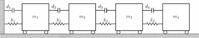
Table 1The parameters of the 4 DOF model
Mass (kg) | Stiffness (N/m) | Damping (N/m) | ||||||||||
Parameter | ||||||||||||
Value | 4 | 5 | 7 | 6 | 500 | 900 | 1200 | 1100 | 35 | 55 | 70 | 45 |
The four DOF lumped parameter system is simulated in Matlab™ using a state-space representation. Defined and identified structural damping matrices are tabulated in Table 2. The results showed that the structural damping matrix identified by the proposed method yields exactly correct values, when the calculated FRFs are employed without adding any noise. However, measurement noise is always present in real engineering problems. Based on the root mean square (RMS) value, 1 % random noise is added to the FRFs of the analytical system to reveal the effects of measurement noise. To give an insight, one of the accelerance FRFs of the system, namely FRF 11, is shown in Fig. 2 in its exact and noisy forms. As it can be seen in Table 2, the damping matrix is estimated almost accurately, despite the presence of 1 % noise. The diagonal terms of the FRF matrix, namely FRF11, FRF22, FRF33 and FRF44 are shown in Fig. 3. The diagonal terms of the normal frequency response function matrix, namely NFRF11, NFRF22, NFRF33 and NFRF44 are given in Fig. 3, as well. The effect of damping on the amplitude of FRFs can be observed clearly in these plots. The phase angles for undamped or proportional damping cases are either 0° or 180°, i.e. the modes are real. This is not the case for non-proportionally damped systems as observed in Fig. 3.
Fig. 2FRF 11 of four DOF lumped parameter model (exact and noisy forms)
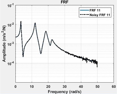
Table 2Defined and estimated structural damping matrices with 0 % noise and with 1 % noise
Defined matrix | Estimated matrix (0% noise) | Estimated matrix (1% noise) | |||||||||
90.0 | –55.0 | 0.0 | 0.0 | 90.0 | –55.0 | 0.0 | 0.0 | 89.0 | –53.7 | –3.7 | 2.7 |
–55.0 | 125.0 | –70.0 | 0.0 | –55.0 | 125.0 | –70.0 | 0.0 | –52.2 | 124.3 | –69.2 | -1.3 |
0.0 | –70.0 | 115.0 | –45.0 | 0.0 | –70.0 | 115.0 | –45.0 | –6.6 | –66.9 | 117.9 | –46.7 |
0.0 | 0.0 | –45.0 | 45.0 | 0.0 | 0.0 | –45.0 | 45.0 | 4.5 | –3.0 | –46.2 | 46.0 |
Fig. 3FRFs and NFRFs of four DOF lumped parameter model with phase angles
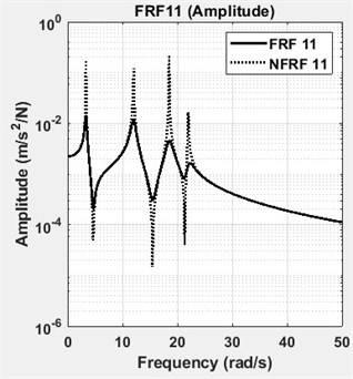
a) FRF11 and NFRF11: amplitude
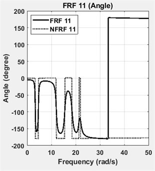
b) FRF11 and NFRF11: angle
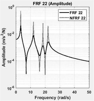
c) FRF22 and NFRF22: amplitude
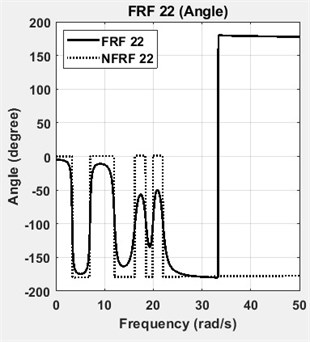
d) FRF22 and NFRF22: angle
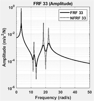
e) FRF33 and NFRF33: amplitude
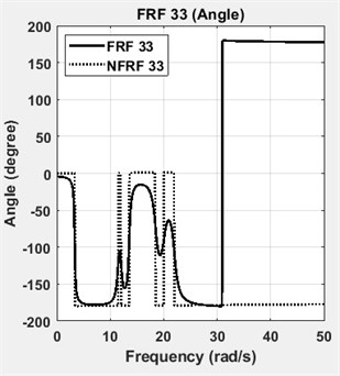
f) FRF33 and NFRF33: angle
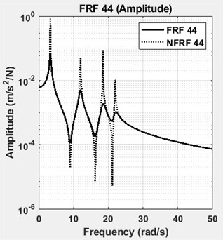
g) FRF44 and NFRF44: amplitude
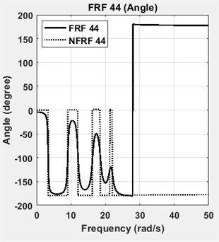
h) FRF44 and NFRF44: angle
The stabilization plot is a further interpretation of the error chart, where stable (i.e. physical) poles are identified as a function of the model order. Identified modal parameters stabilize and converge, when the correct model order is found. The model order is defined as the highest power in a matrix polynomial equation. The poles of the well excited modes are identified at low model orders, whereas the poles of the poorly excited modes will not stabilize, till the model order is increased up to a certain value. The stabilization plots of the analytical model are constructed using Matlab. In Fig. 4, the stabilization plots of four DOF lumped parameter model are given. For a comparison, the stabilization plots of average of four exact FRFs and four noisy FRFs are given separately in Fig. 4(a) and in Fig. 4(b), respectively. Then, all of them are shown in Fig. 4(c), to give an insight about the stabilization calculations. Note that, the number of spectral lines is chosen as 2048 in these calculations.
3. Case study: experimental modal analysis of a test vehicle
Experimental modal analysis (EMA) (a.k.a. modal analysis or modal testing) is the procedure of determining natural frequencies, damping ratios, and mode shapes of a linear time invariant (LTI) system, through vibration testing. Before acquiring experimental data, the excitation and response locations should be determined carefully. In the literature a variety of techniques are available, which addresses the target mode selection, location of sensors and the placement of exciters. An overview of commonly used techniques is given in Ref. [22, 23].
Fig. 4The stabilization plots of four DOF lumped parameter model (# of spectral lines = 2048)
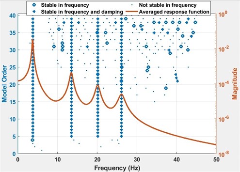
a) The stabilization plot of average of four exact FRFs
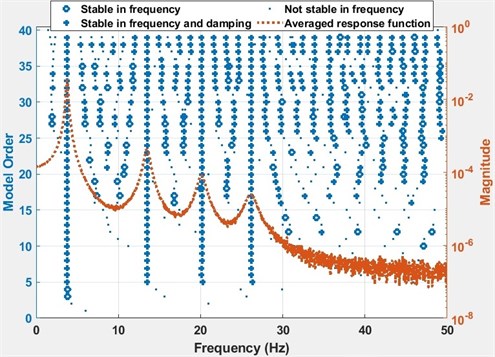
b) The stabilization plot of average of four noisy FRFs
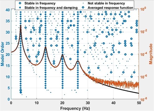
c) The stabilization plot of averages of four exact FRFs and four noisy FRFs
Since it is impossible to instrument a complex structure in all DOFs corresponding to those of the computational model, the experimental data is always spatially incomplete [23]. A reduced model is required to correlate the experimental modal analysis results and the computational analysis results. The most common reduction techniques are: Guyan (static), Generalized Dynamic and SEREP [24, 25]. If the model to be reduced has a huge DOF, Guyan reduction technique is the appropriate one [26]. Guyan reduction is a sub-structuring method, which is commonly used for the solution of computational models with many DOF. In the current study, the computational model is reduced using this technique.
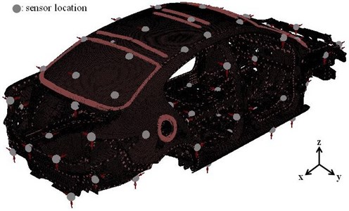
Computational model of the test vehicle is constructed using Altair/Hypermesh™ package [27]. Optimum sensor locations for the EMA study are determined using the modal analysis results of the computational model. In the bandwidth of interest (up to 200 Hz), the number of optimum locations is computed to be 92. These locations are determined by using an optimization algorithm in Siemens LMS VirtualLab™ environment. The algorithm considers the off-diagonal terms of the Auto-MAC matrix. If the off-diagonal terms are smaller than a threshold (usually chosen to be 0.15), the cross-correlation between the modes of interest is low. It means that the modes are spatially well separated [21]. The nodes tagged on the computational model are shown in Fig. 5.
Fig. 5Sensor locations for the experimental modal analysis study. 92 optimum locations are determined by using an optimization algorithm
PCB™ uniaxial accelerometers are located to the determined measurement (output) points. A reduced wireframe model of the test vehicle is constructed by combining the tagged nodes. The reduced model has all the information assigned to the computational model, i.e. material properties, thickness, etc. This reduced model is then used in the correlation and the model updating studies, as well.
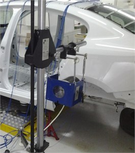
The analyser used in the EMA study is shown in Fig. 6. To excite the structure, Modal Shop™ 2100E11 type electrodynamic shakers are used. To excite both bending and torsional modes, two excitation locations in - and -directions are determined. The determined driving point in -direction is shown in Fig. 7. These driving points are determined after many attempts, where results are monitored with respect to the following criteria [27]:
• Excitation of all structural modes must be achieved in the frequency bandwidth of interest.
• Ordinary coherence value should be read at least 0.7.
Note that, single-input multi-output (SIMO) and multi-input multi-output (MIMO) tests have their own advantages and drawbacks depending on the dynamics of the structure to be tested. There is no single best solution offered for the application of EMA on vehicle structures. Consequently, many test parameters must be reviewed, before attempting to any model updating study. Experimental modal analysis parameters used during the measurements are given in Table 3. For more information about alternative measurement schemes the reader is referred to [27].
FRF measurements should be acquired simultaneously from all the sensor locations. Since the number of analyser channels and sensors were not enough, a roving array of 30 uniaxial accelerometers was employed. To monitor the repeatability of measurements, two reference accelerometers are used throughout the EMA study, as well.
Table 3Experimental modal analysis parameters used during the measurements
Experimental modal analysis parameters | Value |
Number of DOF | 2×92 |
Measurement bandwidth | 512 Hz |
Resolution | 0.5 Hz |
Spectral lines | 1024 |
Excitation signal | Burst random (60 mV) |
Amplifier gain | –4 dB |
Power-law | White noise |
Windowing function | Uniform |
Fig. 6The analyser used in measurements. The photographs are taken at the Automotive Laboratory of Bogazici University
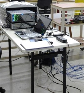
Fig. 7Shaker excitation in y-direction. The photographs are taken at the Automotive Laboratory of Bogazici University
4. Results and discussion
The complex FRFs obtained from the EMA study are refined using digital signal processing techniques. The DOF of the experimental data is 2×92, which means that the modal test is performed using 2 inputs and 92 outputs. In the following equation, the receptance type complex FRF matrix is given:
First two columns of the matrix are populated with the measured FRF data. Due to the reciprocity, it is assumed that the first two rows of the matrix are known, as well. Since the rest of the terms (90×90) are unknown, the receptance matrix is incomplete (symbol “” stands for the unknown terms). The procedure described in ‘analytical solution’ section requires a full (92×92) receptance matrix. To estimate the modal parameters, only one column of the receptance matrix is enough. Next to the identification of the modal parameters of the system, all unknown terms of the receptance matrix can be synthesized to obtain the full matrix.
Measured modal data are processed using the least-squares complex frequency-domain method. Modal parameters are estimated through the measured complex FRFs using Matlab™. The fundamental parameters are complex modal frequencies (), modal vectors () and modal mass (). Current algorithms also extract modal participation vectors () and residues (). The estimation algorithm identifies modal participation vectors. These vectors scale how well each modal vector is excited from each of the driving points determined for the modal test. Combination of the modal participation and modal vectors yields the residue for a mode, i.e.:
Modal participation and modal vectors are supposed to have the information about right and left eigenvectors of a structural mode, respectively [28]. Provided the linear system assumption is hold, the right and the left modal vectors are expected to be proportional to each other. The unknown terms () of the receptance matrix are synthesized using the following equation:
where is mass-normalized modal vector, is angular natural frequency of undamped vibration, is angular frequency of excitation, is structural damping loss factor, is upper residue, is lower residue, is input location, is output location, mode number.
Fig. 8The stabilization plots are calculated using Matlab
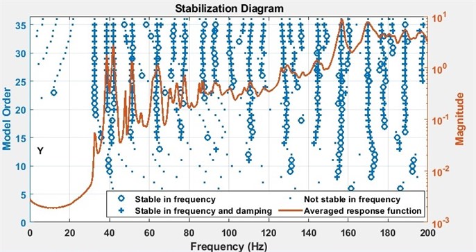
a) The curve is the average of all FRFs measured when the structure is excited in -direction
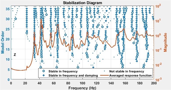
b) The curve is the average of all FRFs measured when the structure is excited in -direction
The second and third members in the right-hand side of Eq. (19) represent the upper and the lower residuals, respectively. The upper and the lower residuals represent the effect of modes, which lie out of the frequency band of interest [29].
In Fig. 8, the stabilization plots of the test vehicle are given: the curves shown in Fig. 8(a) and Fig. 8(b) are the averages of all FRFs measured, when the structure is excited in -direction and -direction, respectively.
Following the same procedure, which is outlined in Section 2, the damping matrix of the structure is populated. Due to the confidentiality of the test results and the size of the matrix only a small part the identified damping values of the structure are given here in Table 4.
Table 4First 12 by 12 part of the identified damping matrix of the structure
8 | –32 | 6 | 23 | –43 | –11 | 49 | –55 | 49 | –35 | 15 | 17 |
–34 | –13 | –38 | 3 | –2 | 4 | –16 | 5 | –3 | 2 | 0 | –1 |
7 | –32 | –12 | –15 | 32 | –18 | 6 | 10 | –21 | 0 | 40 | –6 |
21 | 2 | –14 | –18 | 18 | –40 | 13 | –30 | 4 | –10 | –79 | –50 |
–39 | –3 | 29 | 18 | 16 | –17 | 8 | 4 | 8 | –5 | –36 | 30 |
–12 | 5 | –12 | –41 | –12 | 20 | –18 | –17 | –41 | –3 | 15 | 2 |
51 | –14 | 7 | 14 | 9 | –21 | –1 | –20 | –41 | 58 | 14 | 42 |
–62 | 6 | 11 | –27 | 2 | –16 | –26 | 3 | –21 | 6 | 22 | –35 |
47 | –4 | –24 | 6 | 11 | –49 | –32 | –19 | –1 | 0 | –5 | 5 |
–33 | 1 | –1 | –4 | –6 | –12 | 61 | 4 | –4 | 30 | –88 | 15 |
14 | 1 | 44 | –71 | –42 | 18 | 12 | 27 | –9 | –74 | –7 | 4 |
19 | –2 | –8 | –44 | 36 | 6 | 47 | –29 | 4 | 23 | 7 | –6 |
5. Conclusions
1) Instead of mathematical models based on some assumptions, it is proposed to use the identified structural damping matrix in the computational model.
2) It is shown that the non-proportional structural damping matrix of a system can be identified using Eq. (15) and Eq. (16), where FRFs obtained from EMA are used.
3) A case study is given to demonstrate the application of the proposed procedure.
4) It is shown that once the modal parameters are identified, the unknown terms of the incomplete FRF matrix can readily be synthesized.
5) Most of the modification studies are based on tuning the damping properties of a structure. A reliable damped model is crucial for such studies.
References
-
Baruch M. Optimization procedure to correct stiffness and flexibility matrices using vibration tests. AIAA Journal, Vol. 16, Issue 1, 1978, p. 1208-1210.
-
Berman A., Nagy E. J. Improvement of a large analytical model using test data. AIAA Journal, Vol. 21, Issue 8, 1983, p. 1168-1173.
-
Wei F.-S. Analytical dynamic model improvement using vibration test data. AIAA Journal, Vol. 28, Issue 1, 1990, p. 175-177.
-
Friswell M. I., Inman D., Pilkey D. Direct updating of damping and stiffness matrices. AIAA Journal, Vol. 36, Issue 3, 1998, p. 491-493.
-
Carvalho J., Datta B. N., Gupta A., Lagadapati M. A direct method for model updating with incomplete measured data and without spurious modes. Mechanical Systems and Signal Processing, Vol. 21, Issue 7, 2007, p. 2715-2731.
-
Jacquelin E., Adhikari S., Friswell M. I. A second-moment approach for direct probabilistic model updating in structural dynamics. Mechanical Systems and Signal Processing, Vol. 29, 2012, p. 262-283.
-
Lin R.-M., Ewins D. Model updating using FRF data. Proceedings of the 15th International Seminar on Modal Analysis, 1990, p. 141-162.
-
Kwon K.-S., Lin R.-M. Robust finite element model updating using Taguchi method. Journal of Sound and Vibration, Vol. 280, Issue 1, 2005, p. 77-99.
-
Kim G.-H., Park Y.-S. An automated parameter selection procedure for finite-element model updating and its applications. Journal of Sound and Vibration, Vol. 309, Issue 3, 2008, p. 778-793.
-
Arora V. FE model updating method incorporating damping matrices for structural dynamic modifications. Structural Engineering and Mechanics, Vol. 52, Issue 2, 2014, p. 261-274.
-
Mottershead J. E., Link M., Friswell M. I. The sensitivity method in finite element model updating: A tutorial, Mechanical Systems and Signal Processing, Vol. 25, Issue 7, 2011, p. 2275-2296.
-
Matta E., De Stefano A. Robust finite element model updating of a large-scale benchmark building structure. Structural Engineering and Mechanics, Vol. 43, Issue 3, 2012, p. 371-394.
-
Wang J., Yang Q. Modified Tikhonov regularization in model updating for damage identification. Structural Engineering and Mechanics, Vol. 44, Issue 5, 2012, p. 585-600.
-
Pradhan S., Modak S. Normal response function method for mass and stiffness matrix updating using complex FRFs. Mechanical Systems and Signal Processing, Vol. 32, 2012, p. 232-250.
-
Chen S., Ju M., Tsuei Y. Estimation of mass, stiffness and damping matrices from frequency response functions. Journal of Vibration and Acoustics, Vol. 118, Issue 1, 1996, p. 78-82.
-
Yang Y., Zhao Y., Kang D. Integration on acceleration signals by adjusting with envelopes. Journal of Measurements in Engineering, Vol. 3, Issue 2, 2016, p. 117-121.
-
Oktav A., Yılmaz C., Anlas G. Transfer path analysis: Current practice, trade-offs and consideration of damping. Mechanical Systems and Signal Processing, Vol. 85, 2017, p. 760-772.
-
Lázaro M. Closed form eigensolutions of nonviscously, nonproportionally damped systems based on continuous damping sensitivity. Journal of Sound and Vibration, Vol. 413, 2018, p. 368-382.
-
Lin Ng R. M. T. Y. Frequency response functions and modal analysis of general nonviscously damped dynamic systems with and without repeated modes. Mechanical Systems and Signal Processing, Vol. 120, 2019, p. 744-764.
-
Schilders O. W. H., Van Der Vorst H. A., Rommes J. Model Order Reduction: Theory, Research Aspects and Applications. Berlin, Springer, Vol. 13, 2008.
-
Van Langenhove T., Brughmans M. Using MSC/NASTRAN and LMS/Pretest to find an optimal sensor placement for modal identification and correlation of aerospace structures. LMS International, 1999.
-
Bi Shusheng, et al. Elimination of transducer mass loading effects in shaker modal testing. Mechanical Systems and Signal Processing, Vol. 38, Issue 2, 2013, p. 265-275.
-
Wang Xing, et al. Localisation of local nonlinearities in structural dynamics using spatially incomplete measured data. Mechanical Systems and Signal Processing, Vol. 99, 2018, p. 364-383.
-
Chen G. FE Model Validation for Structural Dynamics. Ph.D. Thesis, University of London, 2001.
-
Davidsson P. Structure-Acoustic Analysis; Finite Element Modelling and Reduction Methods. Ph.D. Thesis, Lund University, 2004.
-
Qingxi, Nong Zhang, Bangji Zhang, Jinchen Ji Boundary condition handling approaches for the model reduction of a vehicle frame. Mechanical Systems and Signal Processing, Vol. 75, 2016, p. 123-137.
-
Oktav A. Experimental and numerical modal analysis of a passenger vehicle. International Journal of Vehicle Noise and Vibration, Vol. 12, Issue 4, 2016, p. 302-313.
-
Pasha H. G., Allemang R. J., Phillips A. W. Techniques for synthesizing FRFs from analytical models. Special Topics in Structural Dynamics, Vol. 6, 2014, p. 73-79.
-
Bilošová A. Modal Testing. Technical Report, Technical University of Ostrava, Czech Republic, 2011.
Cited by
About this article

