Hierarchical sliding mode attitude control of a spherical underwater exploring robot

Liu, Zhimin

doi:10.21595/mme.2020.21252

Mathematical Models in Engineering

Browse Journal

Submit article

Published: 30 June 2020

Check for updates

Hierarchical sliding mode attitude control of a spherical underwater exploring robot

Zhimin Liu¹

¹Shanghai Publishing and Printing College, Shanghai, 200093, China

Cite the article Download PDF

Downloads 961

Abstract

Aiming at the attitude control of the spherical underwater robot, the kinematics and dynamics of the underactuated attitude control adjusting system are analyzed, and its dynamics model is established. By using the differential homeomorphism transformation, the model was divided into two subsystems. Based on the advantages of sliding mode variable structure control, this paper adopts the hierarchical sliding mode variable structure method to design the sliding mode of different variables respectively, and then designs the sliding mode of the whole system. The presented control scheme can solve the coupling problem well. The controller has small overshoot and can well suppress chattering phenomenon. The simulation results show that the designed control law can make the system converge quickly and control the attitude of the underwater spherical robot effectively.

Highlights

The hierarchical sliding mode variable structure method was adopted to design the sliding mode of different variables.
The presented control scheme can solve the coupling problem well.
The controller has small overshoot and can well suppress chattering phenomenon.

1. Introduction

As a kind of special robots, spherical underwater robots have the following advantages: good compression performance, uncoupled hydrodynamic calculation, equal hydrodynamic parameters in each direction. Accordingly, spherical underwater vehicles have a broad prospect of application in underwater archaeological explorations, sea-floor geomorphic observation, aquaculture, and so on [1-3].

Underactuated system has many advantages in practical application. Due to the reduction of the actuators, the weight, cost and volume of the whole control system will be reduced. In a word, the research on the control method of underactuated system has important theoretical and application value [4]. For underactuated vehicles, there were fewer independent motion control actuators than degrees of freedom (DOF) [5]. It has been proven that the underactuated mechanical systems have second-order nonholonomic constraints [6]. The attitude adjusting problem for underactuated underwater vehicles is of great challenge. The famous Brockett’s necessary condition shows that asymptotic stabilization of these underactuated UUVs cannot be achieved with any smooth or continuous time-invariant feedback controllers [7-9]. The underactuated control laws can be used to handle actuator failure for fully-actuated underwater vehicles or over-actuated underwater vehicles [10]. Nowadays, the attitude adjusting problem of underwater vehicles and other rigid underactuated mechanical systems has made some achievements. Throughout the existing research results, the design methods of attitude adjusting controllers include backstepping method [11] and Lyapunov’s direct method [12], sliding mode control [13], adaptive control [14], saturated-state feedback control and model predictive control control [15]. Among these methods, the sliding mode control (SMC) is one of the most effective means to handle the problem of motion control for underactuated underwater vehicles with external disturbance and model uncertainties, because it is natural strong robustness with regard to internal and external disturbance. Moreover, SMC has also the advantages of reduced order, decoupling, fast response, good dynamic characteristics and so on. Therefore, SMC can solve the attitude adjusting problem for underactuated underwater vehicles well.

The traditional SMC is an effective method for dealing with bounded uncertainty/disturbances and parasitic dynamics of nonlinear system. In this paper, a hierarchical sliding mode control method is proposed. The sliding planes of each layer of the method are asymptotically stable, which can drive the underactuated underwater robot to the desired state. Because the sliding mode control has the function of anti-interference, the designed controller in this paper has strong adaptability to all kinds of external disturbances.

2. Physical prototype of BYSQ-2

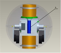
BYSQ-2 underwater spherical robot mainly consists of spherical catheter 1, Sleeve 2, long axis motor 3, weight pendulum 4 and short axis motor 5. Two motors placed perpendicular to each other, which can drive the weight pendulum to rotate to adjust the attitude. Physical prototype of robot is shown in Fig. 1.

Fig. 1Physical prototype of the robot

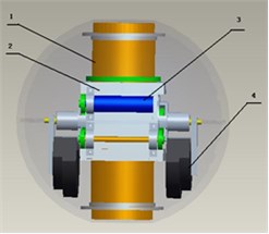
If the components of the underwater spherical robot BYSQ-2 are all regarded as rigid bodies, then BYSQ-2 is a multirigid body composed of three rigid bodies. The spherical shell, catheter and propeller are fixedly connected with each other, which is rigid bodies $B_{1}$ with a total mass $m_{1}$ ; the sleeve is rigid body $B_{2}$ with a mass $m_{2}$ ; the two weightpendulums are called rigid body $B_{3}$ with a mass $m_{3}$ .

3. Kinematic analysis of attitude control system

In order to analyze the motion of multi rigid body system of underwater spherical robot, the following four coordinate systems are established {0}, {1}, {2}, {3}, as shown in Fig. 2.

Fig. 2Coordinate system diagram of multi rigid body system of underwater spherical robot

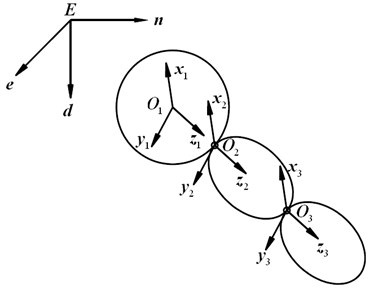
The coordinate system {0} is an inertial reference system fixed to the earth, with the $E n$ axis pointing north and the $E d$ axis pointing vertically downward; the coordinate system {1} is a dynamic reference system fixed to the rigid body $B_{1}$ , with the origin at the center of the ball, the $O_{1} x_{1}$ axis along the long axis, initially parallel to the coordinate system {0}, and the $O_{1} x_{1}$ axis coincides with the axis; the coordinate system {2} is fixed to the rigid body $B_{2}$ , with the origin at the center of the ball, the $O_{2} x_{2}$ axis along the long axis, the coordinate system {3} is fixed to the rigid body $B_{3}$ and the origin is located at the center of the ball. At the beginning, the coordinate system {3} is parallel to the coordinate system {2} and the $O_{3} x_{3}$ axis coincides with the axis $O_{2} x_{2}$ .

Because the Euler angles of the body coordinate system {1} and the relative inertia coordinate system {0} are respectively $ϕ$ , $θ$ and $ψ$ , let:

1

\{\begin{array}{l} z_{1} = ϕ, \\ z_{2} = θ, \\ z_{3} = ψ . \end{array}

Then the angular velocity $ω_{0}$ and acceleration $ε_{0}$ of the coordinate system {1} relative to the coordinate system {0} are:

2

ω_{0} = [\begin{array}{l} {\dot{z}}_{1} \\ {\dot{z}}_{2} \\ {\dot{z}}_{3} \end{array}], ε_{0} = [\begin{array}{l} {\ddot{z}}_{1} \\ {\ddot{z}}_{2} \\ {\ddot{z}}_{3} \end{array}]

Because the angular velocity of the rigid body around the axis $x_{1}$ is $p$ , the angular velocity in the axis $O_{1} y_{1}$ direction is $q$ , and the angular velocity in the axis $z_{1}$ direction is $r$ .

Let:

3

\{\begin{array}{l} z_{4} = p, \\ z_{5} = q, \\ z_{6} = r . \end{array}

It can be concluded that the angular velocity $ω_{1}$ and acceleration of the rigid body $ε_{1}$ in the body coordinate system {1} are:

4

ω_{1} = [\begin{array}{l} z_{4} \\ z_{5} \\ z_{6} \end{array}], ε_{1} = [\begin{array}{l} {\dot{z}}_{4} \\ {\dot{z}}_{5} \\ {\dot{z}}_{6} \end{array}] .

The relationship between the angular velocity of the rigid body $B_{1}$ in relative inertial coordinate system {0} and the body coordinate system {1} is as follows:

5

\begin{array}{l} \dot{ϕ} = p + q s i n ϕ t a n θ + r c o s ϕ t a n θ, \\ \dot{θ} = q c o s ϕ - r s i n ϕ, \\ \dot{ψ} = q \frac{s i n ϕ}{c o s θ} + r \frac{c o s ϕ}{c o s θ} . \end{array}

Let the rotation angle of coordinate system {2} relative to axis $O_{1} x_{1}$ of coordinate system {1} be $α$ , The attitude transformation matrix can be obtained as:

6

[\begin{array}{l} 1 & 0 & 0 \\ 0 & c o s α & - s i n α \\ 0 & s i n α & c o s α \end{array}] .

Let the angular velocity of the rigid body $B_{2}$ around the axis $O_{2} x_{2}$ is $z_{7}$ , then:

7

\dot{α} = z_{4} + z_{7} .

And let:

8

z_{8} = α .

Let the rotation angle of coordinate system {3} relative to axis $O_{2} y_{2}$ of coordinate system {2} be $β$ , the angular velocity of the rigid body $B_{3}$ around the axis $y_{3}$ is $z_{9}$ , then:

9

\dot{β} = z_{5} + z_{9} .

The attitude transformation matrix can be obtained as:

10

[\begin{array}{l} 1 & 0 & t a n β \\ 0 & 1 & 0 \\ 0 & 0 & \frac{1}{c o s β} \end{array}] .

4. Dynamic analysis of attitude control system

According to the dynamic model equation of the underwater spherical robot established by Fossen [16], the dynamic equation of the rigid body $B_{1}$ when the propeller is not working can be obtained as follows:

11

\begin{array}{l} I_{1 x} \dot{p} + (I_{1 z} - I_{1 y}) q r - (\dot{r} + p q) I_{1 x z} + (r^{2} - q^{2}) I_{1 y z} + (p r - \dot{q}) I_{1 x y} = M_{1}, \\ I_{1 y} \dot{q} + (I_{1 x} - I_{1 z}) r p - (\dot{p} + q r) I_{1 x y} + (p^{2} - r^{2}) I_{1 z x} + (p q - \dot{r}) I_{1 y z} = M_{2 y}^{'}, \\ I_{1 z} \dot{r} + (I_{1 y} - I_{1 x}) p q - (\dot{q} + r p) I_{1 y z} + (q^{2} - p^{2}) I_{1 x y} + (r q - \dot{p}) I_{1 x z} = M_{2 z}^{'}, \end{array}

where $I_{1 x}$ , $I_{1 y}$ , $I_{1 z}$ are the moment of inertia of the rigid body $B_{1}$ around the $O_{1} x_{1}$ axis, $O_{1} y_{1}$ axis and $O_{1} z_{1}$ axis respectively. $M_{2 y}^{'}$ and $M_{2 z}^{'}$ are the components of the torque of the short axis motor acting on the rigid body on the $O_{1} y_{1}$ axis and $O_{1} z_{1}$ axis. $I_{1 x y}$ , $I_{1 x z}$ and $I_{1 y z}$ are the inertial products of rigid body $B_{1}$ to plane $x_{1} o_{1} y_{1}$ , $x_{1} o_{1} z_{1}$ and $y_{1} o_{1} z_{1}$ , respectively and:

12

\begin{array}{l} I_{1 x} = \int_{Ω} ρ (y^{2} + z^{2}) d x d y d z, \\ I_{1 y} = \int_{Ω} ρ (x^{2} + z^{2}) d x d y d z, \\ I_{1 z} = \int_{Ω} ρ (x^{2} + y^{2}) d x d y d z, \end{array}

13

\begin{array}{l} I_{1 x y} = \int_{Ω} ρ x y d x d y d z, \\ I_{1 x z} = \int_{Ω} ρ x z d x d y d z, \\ I_{1 y z} = \int_{Ω} ρ y z d x d y d z . \end{array}

Due to the symmetry of the structure, we have:

14

\begin{array}{l} I_{1 y} = I_{1 z}, \\ I_{1 x y} = I_{1 x z} = I_{1 y z} = 0 . \end{array}

Since the values of $I_{x}$ are similar to those of $I_{y}$ and $I_{z}$ , it is considered that:

15

I_{1 x} = I_{1 y} = I_{1 z} .

So Eq. (11) can be reduced to:

16

\begin{array}{l} I_{1 x} \dot{p} = M_{1}, \\ I_{1 y} \dot{q} = M_{2 y}^{'}, \\ I_{1 z} \dot{r} = M_{2 z}^{'}, \end{array}

where $I_{2 y}$ and $I_{2 z}$ are the moment of inertia of the sleeve (rigid body $B_{2}$ ) around the $O_{2} y_{2}$ axis and $O_{2} z_{2}$ axis respectively.

Due to the regular shape of the sleeve, it can be approximately considered that:

17

I_{2 y} = I_{2 z} = I_{2 y z},

where $I_{2 y z}$ is the moment of inertia of the sleeve (rigid body $B_{2}$ ) about any axis in the plane.

And we have:

18

\begin{array}{l} I_{1 x} \dot{p} = M_{1}, \\ (I_{1 y} + I_{2 y z}) \dot{q} = M_{2 y}^{'}, \\ (I_{1 z} + I_{2 y z}) \dot{r} = M_{2 z}^{'} . \end{array}

Let:

19

\begin{array}{l} I_{y}^{'} = I_{1 y} + I_{2 y}, \\ I_{z}^{'} = I_{1 z} + I_{2 z} . \end{array}

Since:

20

I_{1 y} = I_{1 z} .

We have:

21

I_{y}^{'} = I_{z}^{'} .

Then the system model Eq. (16) can be rewritten as:

22

\begin{array}{l} I_{1 x} \dot{p} = M_{1}, \\ I_{y}^{'} \dot{q} = M_{2 y}^{'}, \\ I_{z}^{'} \dot{r} = M_{2 z}^{'} . \end{array}

In the coordinate system {3}, the torque of short axis motor can be expressed as:

23

[\begin{matrix} 0 \\ M_{2} \\ 0 \end{matrix}] .

$M_{2 y}^{'}$ and $M_{2 z}^{'}$ can be expressed as:

24

\begin{array}{l} [\begin{array}{l} 0 \\ M_{2 y}^{'} \\ M_{2 z}^{'} \end{array}] = [\begin{array}{l} 1 & 0 & 0 \\ 0 & c o s α & - s i n α \\ 0 & s i n α & c o s α \end{array}] [\begin{array}{l} 1 & 0 & t a n β \\ 0 & 1 & 0 \\ 0 & 0 & \frac{1}{c o s β} \end{array}] [\begin{matrix} 0 \\ M_{2} \\ 0 \end{matrix}] = [\begin{matrix} 0 \\ M_{2} c o s α \\ M_{2} s i n α \end{matrix}] \end{array} .

Then Eq. (22) can be reduced to:

25

\begin{array}{l} \dot{p} = \frac{M_{1}}{I_{1 x}}, \\ \dot{q} = \frac{M_{2} c o s α}{I_{1 y} + I_{2 y}} \\ \dot{r} = \frac{M_{2} s i n α}{I_{1 z} + I_{2 z}} . \end{array},

Let:

26

k_{1} = \frac{1}{I_{1 x}}, k_{2} = \frac{1}{I_{1 y} + I_{2 y}}, k_{3} = k_{2} = \frac{1}{I_{1 z} + I_{2 z}}, k_{4} = \frac{1}{I_{2 x} + I_{3 x}} .

Then make the input transformation, let:

27

\begin{array}{l} τ_{1} = M_{1}, \\ τ_{2} = M_{2} . \end{array}

Then the state equation of the spherical shell attitude control system is:

28

\begin{array}{l} {\dot{z}}_{1} = z_{4} + z_{5} s i n z_{1} t a n z_{2} + z_{6} c o s z_{1} t a n z_{2}, \\ {\dot{z}}_{2} = z_{5} c o s z_{1} - z_{6} s i n z_{1}, \\ {\dot{z}}_{3} = z_{5} \frac{s i n z_{1}}{c o s z_{2}} + z_{6} \frac{c o s z_{1}}{c o s z_{2}}, \\ {\dot{z}}_{4} = k_{1} τ_{1}, \\ {\dot{z}}_{5} = k_{2} τ_{2} c o s z_{8}, \\ {\dot{z}}_{6} = k_{3} τ_{2} s i n z_{8}, \\ {\dot{z}}_{7} = - 2 k_{4} τ_{1}, \\ {\dot{z}}_{8} = z_{4} + z_{7} . \end{array}

Further simplifying Eqs. (6-28), we can get:

29

\begin{array}{l} {\ddot{z}}_{1} - {\ddot{z}}_{3} s i n z_{2} - {\dot{z}}_{2} {\dot{z}}_{3} c o s z_{2} = k_{1} τ_{1}, \\ {\ddot{z}}_{2} c o s z_{1} + {\ddot{z}}_{3} s i n z_{1} c o s z_{2} + {\dot{z}}_{1} {\dot{z}}_{3} c o s z_{1} c o s z_{2} - {\dot{z}}_{1} {\dot{z}}_{2} s i n z_{1} - {\dot{z}}_{2} {\dot{z}}_{3} s i n z_{1} s i n z_{2} = k_{2} τ_{2} c o s z_{8}, \\ - {\ddot{z}}_{2} s i n z_{1} + {\ddot{z}}_{3} c o s z_{1} c o s z_{2} - {\dot{z}}_{1} {\dot{z}}_{3} s i n z_{1} c o s z_{2} - {\dot{z}}_{1} {\dot{z}}_{2} c o s z_{1} - {\dot{z}}_{2} {\dot{z}}_{3} c o s z_{1} s i n z_{2} = k_{3} τ_{2} s i n z_{8}, \\ {\ddot{z}}_{8} = (k_{1} - 2 k_{4}) τ_{1} . \end{array}

Let:

30

[\begin{array}{l} ε_{11} \\ ε_{21} \\ ε_{31} \\ ε_{41} \end{array}] = [\begin{array}{l} z_{1} \\ z_{2} \\ z_{3} \\ z_{8} \end{array}] .

Considering modeling error and external interference, from Eq. (29), we can obtain:

31

\begin{array}{l} {\dot{ε}}_{11} = ε_{12}, {\dot{ε}}_{12} = f_{1} (ε) + F_{1} (ε) τ_{2} + k_{1} τ_{1} + d_{1}, \\ {\dot{ε}}_{21} = ε_{22}, {\dot{ε}}_{22} = f_{2} (ε) + F_{2} (ε) τ_{2} + d_{2}, \\ {\dot{ε}}_{31} = ε_{32}, {\dot{ε}}_{32} = f_{3} (ε) + F_{3} (ε) τ_{2} + d_{3}, \\ {\dot{ε}}_{41} = ε_{42}, {\dot{ε}}_{42} = (k_{1} - 2 k_{4}) τ_{1}, \end{array}

where $d_{1}$ , $d_{2}$ and $d_{3}$ are modeling errors and external disturbances, and

f_{1} (ε) = ε_{12} ε_{22} t a n ε_{21} + ε_{22} ε_{32} s i n ε_{21} t a n ε_{21} + ε_{22} ε_{32} c o s ε_{21},

f_{2} (ε) = - ε_{12} ε_{32} s i n ε_{21}, f_{3} (ε) = \frac{ε_{12} ε_{22}}{c o s ε_{21}} + ε_{22} ε_{32} t a n ε_{21},

F_{1} (ε) = k_{2} t a n ε_{21} (s i n ε_{11} c o s ε_{41} + c o s ε_{11} s i n ε_{41}),

F_{2} (ε) = k_{2} (c o s ε_{11} c o s ε_{41} - s i n ε_{11} s i n ε_{41}),

F_{3} (ε) = \frac{k_{2}}{c o s ε_{21}} (s i n ε_{11} c o s ε_{41} + c o s ε_{11} s i n ε_{41}) .

Since the values of $ε_{41}$ and $ε_{42}$ are only two state variables needed in the design of control system, and there is no expected value, Eqs. (6-31) can be simplified to:

32

\begin{array}{l} {\dot{ε}}_{11} = ε_{12}, \\ {\dot{ε}}_{12} = f_{1} (ε) + F_{1} (ε) τ_{2} + k_{1} τ_{1} + d_{1}, \\ {\dot{ε}}_{21} = ε_{22}, \\ {\dot{ε}}_{22} = f_{2} (ε) + F_{2} (ε) τ_{2} + d_{2}, \\ {\dot{ε}}_{31} = ε_{32}, \\ {\dot{ε}}_{32} = f_{3} (ε) + F_{3} (ε) τ_{2} + d_{3} . \end{array}

5. Control design

To design the control law conveniently, the system Eq. (32) is divided into two subsystems:

33

\begin{array}{l} \sum_{1} \{\begin{array}{l} {\dot{ε}}_{21} = ε_{22}, \\ {\dot{ε}}_{22} = f_{2} (ε) + F_{2} (ε) τ_{2} + d_{2}, \\ {\dot{ε}}_{31} = ε_{32}, \\ {\dot{ε}}_{32} = f_{3} (ε) + F_{3} (ε) τ_{2} + d_{3}, \end{array} \\ \sum_{2} \{\begin{array}{l} {\dot{ε}}_{11} = ε_{12}, \\ {\dot{ε}}_{12} = f_{1} (ε) + F_{1} (ε) τ_{2} + k_{1} τ_{1} + d_{1} . \end{array} \end{array}

Then the back stepping sliding mode control law is designed for the two subsystems respectively.

Firstly, for the system $\sum_{1},$ the position error of the system is:

34

\{\begin{array}{l} e_{2} = ε_{21} - ε_{21 d}, \\ e_{3} = ε_{31} - ε_{31 d} . \end{array}

The sliding mode function can be designed as:

35

\{\begin{array}{l} s_{2} = c_{2} e_{2} + {\dot{e}}_{2}, \\ s_{3} = c_{3} e_{3} + {\dot{e}}_{3}, \end{array}

where $c_{2}$ and $c_{3}$ are positive constants.

From Eq. (31), we have:

36

\begin{array}{l} {\dot{e}}_{2} = {\dot{ε}}_{21} - {\dot{ε}}_{21 d} = ε_{22}, \\ {\ddot{e}}_{2} = {\ddot{ε}}_{21} - {\ddot{ε}}_{21 d} = f_{2} (ε) + F_{2} (ε) τ_{2} + d_{2}, \\ {\dot{e}}_{3} = {\dot{ε}}_{31} - {\dot{ε}}_{31 d} = ε_{32}, \\ {\ddot{e}}_{3} = {\ddot{ε}}_{31} - {\ddot{ε}}_{31 d} = f_{3} (ε) + F_{3} (ε) τ_{2} + d_{3}, \end{array}

and

37

\begin{array}{l} s_{2} = c_{2} (ε_{21} - ε_{21 d}) + ε_{22}, \\ {\dot{s}}_{2} = c_{2} ({\dot{ε}}_{21} - {\dot{ε}}_{21 d}) + {\dot{ε}}_{22} = c_{2} ε_{22} + f_{2} (ε) + F_{2} (ε) τ_{2} + d_{2}, \\ s_{3} = c_{3} (ε_{31} - ε_{31 d}) + ε_{32}, \\ {\dot{s}}_{3} = c_{3} ({\dot{ε}}_{31} - {\dot{ε}}_{31 d}) + {\dot{ε}}_{22} = c_{3} ε_{32} + f_{3} (ε) + F_{3} (ε) τ_{2} + d_{3} . \end{array}

If the following control laws are designed:

38

\{\begin{array}{l} τ_{21} = \frac{1}{F_{2} (ε)} (- c_{2} ε_{22} - f_{2} (ε) - D_{2} s g n (s_{2})), \\ τ_{22} = \frac{1}{F_{3} (ε)} (- c_{3} ε_{32} - f_{3} (ε) - D_{3} s g n (s_{3})), \end{array}

where $D_{2}$ is the upper bound of $d_{2}$ , $D_{3}$ is the upper bound of $d_{3}$ , sgn represented symbolic function, its definition is given by:

39

\{\begin{array}{l} s g n (s) = + 1, s > 0, \\ s g n (s) = - 1, s < 0 . \end{array}

Substituting Eqs. (38) and (39) into Eq. (37),we have:

40

\begin{array}{l} {\dot{s}}_{2} = - D_{2} s g n (s_{2}) + d_{2}, \\ {\dot{s}}_{3} = - D_{3} s g n (s_{3}) + d_{3}, \end{array}

and

41

\{\begin{array}{l} s_{2} {\dot{s}}_{2} = s_{2} (- D_{2} s g n (s_{2}) + d_{2}) = - D_{2} |s_{2}| + d_{2} s_{2} \leq 0, \\ s_{3} {\dot{s}}_{3} = s_{3} (- D_{3} s g n (s_{3}) + d_{3}) = - D_{3} |s_{3}| + d_{3} s_{3} \leq 0 . \end{array}

Due to the coupling effect between the two subsystems in the system, it is not reasonable to add the two control laws easily, and we need to introduce the control law corresponding to the coupling effect.

The total desired control law is set to:

42

τ_{2} = τ_{21} + τ_{22} + τ_{2 h},

where $τ_{2 h}$ is the coupled switching control law of the system in approach stage.

Now we construct the second sliding plane:

43

S = C s_{2} + s_{3},

where $C$ is a positive constant.

To get the coupled switching control law, the CLF is chosen as:

44

V_{1} = \frac{1}{2} S^{2},

the first-order time-derivative of the CLF $V_{1}$ renders to:

45

{\dot{V}}_{1} = S \dot{S} = S (C {\dot{s}}_{2} + {\dot{s}}_{3}),

substituting Eqs. (37) into Eq. (45), we have:

46

{\dot{V}}_{1} = S ((C F_{2} (ε) τ_{22} + F_{3} (ε) τ_{21}) + (C F_{2} (ε) + F_{3} (ε)) τ_{2 h}) .

If the exponential approach law is taken for the system from the initial state to the switching surface, then:

47

(C F_{2} (ε) τ_{22} + F_{3} (ε) τ_{21}) + (C F_{2} (ε) + F_{3} (ε)) τ_{2 h} = - p_{1} s g n (S) - p_{2} S,

where $p_{1}$ and $p_{2}$ are positive constants.

From Eq. (47), we have:

48

τ_{2 h} = - \frac{1}{C F_{2} (ε) + F_{3} (ε)} (C F_{2} (ε) τ_{22} + F_{3} (ε) τ_{21} + p_{1} s g n (S) + p_{2} S),

and

49

{\dot{V}}_{1} = - p_{1} |S| - p_{2} S^{2} \leq 0,

50

τ_{2} = τ_{21} + τ_{22} + τ_{2 h} = \frac{1}{C F_{2} (ε) + F_{3} (ε)} (F_{3} (ε) τ_{22} + C F_{2} (ε) τ_{21} - p_{1} s g n (S) - p_{2} S)

= \frac{- 1}{C F_{2} (ε) + F_{3} (ε)} (c_{3} ε_{32} + f_{3} (ε) + D_{3} s g n (s_{3}) + C c_{2} ε_{22} + C f_{2} (ε) + C D_{2} s g n (s_{2}) + p_{1} s g n (S) + p_{2} S) .

Secondly, for system $\sum_{2},$ the position error of the system is:

51

e_{1} = ε_{11} - ε_{11 d} .

The sliding mode function is chosen by the following equation:

52

s_{1} = c_{1} e_{1} + {\dot{e}}_{1},

where $c_{1}$ is a positive constant.

From Eq. (31), we have:

53

\begin{array}{l} {\dot{e}}_{1} = {\dot{ε}}_{11} - {\dot{ε}}_{11 d} = ε_{12}, \\ {\ddot{e}}_{1} = {\ddot{ε}}_{11} - {\ddot{ε}}_{11 d} = f_{1} (ε) + F_{1} (ε) τ_{2} + k_{1} τ_{1}, \end{array}

and

54

\{\begin{array}{l} s_{1} = c_{1} (ε_{11} - ε_{11 d}) + ε_{12}, \\ {\dot{s}}_{1} = c_{1} ({\dot{ε}}_{11} - {\dot{ε}}_{11 d}) + {\dot{ε}}_{12} = c_{1} ε_{12} + f_{1} (ε) + F_{1} (ε) τ_{2} + k_{1} τ_{1} . \end{array}

Let us definite the following Lyapunov function:

55

V_{2} = V_{1} + \frac{1}{2} s_{1}^{2} .

If the exponential approach law is taken for the system from the initial state to the switching surface, then:

56

c_{1} ε_{12} + f_{1} (ε) + F_{1} (ε) τ_{2} + k_{1} τ_{1} = - p_{1}^{'} s g n (s_{1}) - p_{2}^{'} s_{1},

where $p_{1}^{'}$ and $p_{2}^{'}$ are positive constants.

From Eq. (56), the control input $τ_{1}$ can be obtained as:

57

τ_{1} = - \frac{1}{k_{1}} (p_{1}^{'} s g n (s_{1}) + p_{2}^{'} s_{1} + c_{1} ε_{12} + f_{1} (ε) + F_{1} (ε) τ_{2}),

and

58

{\dot{V}}_{2} = {\dot{V}}_{1} + s_{1} {\dot{s}}_{1} = {\dot{V}}_{1} - p_{1}^{'} |s_{1}| - p_{2}^{'} {s_{1}}^{2} \leq 0 .

According to the aforementioned discussion, it is known that the control law Eqs. (50), (57) can drive arbitrary tracking errors to converge to the origin.

6. Simulation

According to the designed hierarchical sliding mode control law, we carry out some computer simulations by using the Simulink box to demonstrate the performance of the designed controller. The initial attitude value ( $ϕ, θ, ψ$ ) of the rigid body $B_{1}$ is ( $π / 2, π / 4, π / 4$ ). The desired attitude value ( $ϕ_{d}, θ_{d}, ψ_{d}$ ) of the rigid body $B_{1}$ is ( $π / 6, π / 3, π / 2$ ). The parameters are selected as follows: $c_{1} = 48$ , $c_{2} = 60$ , $c_{3} = 80$ , $C = 96$ , $p_{1} = 8$ , $p_{2} = 9$ , $p_{1}^{'} = 7$ , $p_{2}^{'} = 12$ .

The modeling errors and interferences are selected as follows: $D_{1} =$ 0.2, $D_{2} =$ 0.1, $D_{3} =$ 0.3.

Fig. 3Change of roll angle

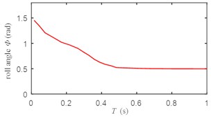
Fig. 4Change of pitch angle

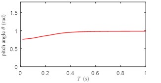
Fig. 5Change of yaw angle

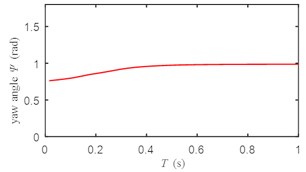
Fig. 6Input torque change of long axis motor

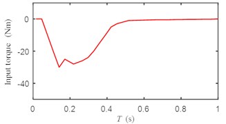
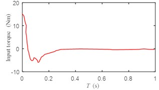
Fig. 7Input torque change of short axis motor

According to Figs. 3-5, the response curves of roll angle, pitch angle and yaw angle have no oscillation, the rise time is less than 0.6 s, the transition time is less than 1 s, and the system has good dynamic performance.

According to Fig. 6, the input torque of the long axis motor has a small chattering, but does not affect the output of the system.

According to Fig. 7, the input torque of the short axis motor have no chatter.

In order to further test the performance of the controller, we carried out a circular experiment. The expected trajectory of the underwater spherical robot is an arc with a radius of 0.5 m, that is $x_{d} =$ 0.5 m, $y_{d} =$ 0.5 m, the initial value of ( $x$ , $y$ , $θ$ ) is (0, 0.5, 0). The value of $θ$ is from 0 to $π / 2$ . The disturbance of the current can be expressed as $τ_{w} = 0.6 + 0.8 s i n (0.8 t + π / 4)$ .

The simulation results are shown in Figs. 8-11.

Fig. 8Change of the yaw angle

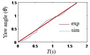
Fig. 9Change of y

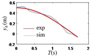
Fig. 10Change of x

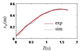
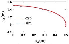
Fig. 11Trajectory of the robot

According to Figs. 8-9, the absolute value of heading angle error is less than 0.2 rad, the absolute value of horizontal position error is less than 0.10 m, and the absolute value of vertical position error is less than 0.08 m.

According to Figs. 10-11, the trajectory of the underwater spherical robot is an arc with an approximate radius of 0.5 m.

Therefore, the experimental results show that the established dynamic control law based on this model are effective, which can realize the tracking of the motion track in the vertical plane, The controller has small overshoot and can well suppress chattering phnomenon and the control accuracy is ideal.

The above simulation results show the feasibility of the hierarchical sliding mode control law in the attitude adjusting control of the underwater spherical robot.

References

Guo Shuxiang, Du Juan, Ye Xiufen, Gao Hongtao, Gu Yizhou Real-time adjusting control algorithm for the spherical underwater robot. International Journal on Information, Vol. 13, 2010, p. 2021-2029.

Search CrossRef
Li Yansheng, Yang Meimei, Sun Hanxu Fluctuation characteristics and rolling control for an underactuated spherical underwater exploration robot. Journal of Vibroengineering, Vol. 19, Issue 2, 2017, p. 1050-1061.

Publisher
Gu Shuoxin, Guo Shuxiang Performance evaluation of a novel propulsion system for the spherical underwater robot (SURIII). Applied Sciences, Vol. 7, 2017, p. 1196.

Publisher
Seifried R. Dynamics of Underactuated Multibody Systems: Modeling, Control and Optimal Design. Solid Mechanics and Its Applications, Springer International Publishing, 2014.

Publisher
Shojaei K. Neural adaptive robust control of underactuated marine surface vehicles with input aturation. Applied Ocean Research, Vol. 53, 2015, p. 267-278.

Publisher
Sabiha Wadoo, Pushkin Kachroo Autonomous Underwater Vehicles Modeling, Control Design and Simulation. CRC Press, 2011.

Search CrossRef
Brockett R. W. Asymptotic Stability and Feedback Stabilization. Differential Geometric Control Theory, Birkhauser, 1993.

Search CrossRef
Bhat S. P., Bernstein D. S. Finite-time stability of homogeneous systems. Proceedings of the American Control Conference, Albuquerque, New Mexico, USA, 1997, p. 2514-2513.

Search CrossRef
Bhat S. P., Bernstein D. S. Finite-time stability of continuous autonomous systems. SIAM Journal on Control and Optimization, Vol. 38, Issue 3, 2000, p. 751-766.

Publisher
Yu Haomiao, Guo Chen, Yan Zheping Globally finite-time stable three-dimensional trajectory-tracking control of underactuated UUVs. Ocean Engineering, Vol. 189, 2019, p. 106329.

Publisher
Pettersen K. Y., Egeland O. Position and attitude control of an underactuated autonomous underwater vehicle. Proceedings of 35th IEEE Conference on Decision and Control, 1996.

Publisher
Hua M. D., Hamel T., Morin P., et al. Control of thrust-propelled underactuated vehicles. IEEE International Conference on Robotics and Automation, 2008.

Search CrossRef
Jun B.-H., Park J.-Y., Lee F.-Y. Development of the AUV ‘ISiMI’ and free running test in an ocean engineering basin. Ocean Engineering, Vol. 36, Issue 1, 2009, p. 2-14.

Publisher
Isa K., Arshad M. R., Ishak S. A hybrid-driven underwater glider model, hydrodynamics estimation, and an analysis of the motion control. Ocean Engineering, Vol. 81, Issue 2, 2014, p. 111-129.

Publisher
Lin W., Chin C. S. Block diagonal dominant remotely operated vehicle model simulation using decentralized model predictive control. Advances in Mechanical Engineering, Vol. 9, Issue 4, 2017, https://doi.org/10.1177/1687814017698886.

Publisher
Fossen T. I. Handbook of Marine Craft Hydrodynamics and Motion Control. 1st. Edition, Wiley, 2011.

Publisher

About this article

Received

20 December 2019

Accepted

31 March 2020

Published

30 June 2020

DOI

https://doi.org/10.21595/mme.2020.21252

Keywords

spherical underwater exploring robot

hierarchical sliding mode

attitude control underactuated system

Acknowledgements

The authors would like to thank the support of China National Natural Science Foundation (51175048) for the research.

This is an open access article distributed under the Creative Commons Attribution License, which permits unrestricted use, distribution, and reproduction in any medium, provided the original work is properly cited.

Previous article in issue Previous Next article in issue Next

Research article

2017 12 01

Research and analysis of spherical magnetic drive for attitude control on nano satellites

Gražvydas Kazokaitis, Vytautas Jūrėnas, Darius Eidukynas

Research article

2017 03 31

Fluctuation characteristics and rolling control for an underactuated spherical underwater exploration robot

Yansheng Li, Meimei Yang, Hanxu Sun, Zhimin Liu

Research article

2016 09 30

Finite time point-stabilization of underwater spherical roving robot

Zhimin Liu, Hanxu Sun, Yansheng Li, Qingxuan Jia, Ming Chu

Research article

2014 09 30

Experiment, simulation and analysis on coupling hydrodynamic forces under key parameters for a spherical underwater exploration robot

Yansheng Li, Hanxu Sun, Ming Chu, Yanheng Zhang, Qingxuan Jia, Xiaojuan Lan

Z. Liu, “Hierarchical sliding mode attitude control of a spherical underwater exploring robot,” Mathematical Models in Engineering, Vol. 6, No. 2, pp. 122–133, Jun. 2020, https://doi.org/10.21595/mme.2020.21252

Copy Extrica

Copied to clipboard!

TY  - JOUR
DO  - 10.21595/mme.2020.21252
UR  - https://doi.org/10.21595/mme.2020.21252
TI  - Hierarchical sliding mode attitude control of a spherical underwater exploring robot
T2  - Mathematical Models in Engineering
AU  - Liu, Zhimin
PY  - 2020
DA  - 2020/06/30
PB  - JVE International Ltd.
SP  - 122-133
IS  - 2
VL  - 6
SN  - 2351-5279
SN  - 2424-4627
ER  - 

Copy Ris

Copied to clipboard!

@article{Liu_2020,
	doi = {10.21595/mme.2020.21252},
	url = {https://doi.org/10.21595/mme.2020.21252},
	year = 2020,
	month = {jun},
	publisher = {{JVE} International Ltd.},
	volume = {6},
	number = {2},
	pages = {122--133},
	author = {Zhimin Liu},
	title = {Hierarchical sliding mode attitude control of a spherical underwater exploring robot},
	journal = {Mathematical Models in Engineering}
}

Copy Bibtex

Copied to clipboard!

[1]Z. Liu, “Hierarchical sliding mode attitude control of a spherical underwater exploring robot,” Mathematical Models in Engineering, vol. 6, no. 2, pp. 122–133, Jun. 2020, doi: 10.21595/mme.2020.21252.

Copy IEEE

Copied to clipboard!

Liu, Zhimin. “Hierarchical Sliding Mode Attitude Control of a Spherical Underwater Exploring Robot.” Mathematical Models in Engineering 6, no. 2 (June 30, 2020): 122–33. https://doi.org/10.21595/mme.2020.21252.

Copy Chicago

Copied to clipboard!

Hierarchical sliding mode attitude control of a spherical underwater exploring robot

Abstract

Highlights

1. Introduction

2. Physical prototype of BYSQ-2

3. Kinematic analysis of attitude control system

4. Dynamic analysis of attitude control system

5. Control design

6. Simulation

References

About this article

Related Articles