Abstract
This article presents the structural health analysis of a full-scale vehicular bridge, using a twin model calibrated with experimental information. This structure consists of concrete arches, built more than 80 years ago, and reinforced in the 1990s with a steel structure. Different load combinations were evaluated in this model to determine the strength of the structure according to current design standards. Finally, it was found that several of its components do not meet the current design requirements, putting the structure in a vulnerable condition to seismic hazards and restricting its service to traffic loads.
1. Introduction
Bridges are a vital component of any transport network [1]. The proper performance of these structures provides a foundation on which the economy of a region can be grown. However, these structures are continuously subjected to different types of dynamic loads, such as traffic, wind and earthquake. These loads can produce excessive vibrations in the structure, causing damage to its components, limiting its service and making its users uncomfortable [2].
The control of structural vibrations is one of the main objectives of the design process. Based on this, minimum material specifications, boundary conditions and geometry of structural components are defined [3]. However, the actual behavior of the structure can differ significantly from the initial design, especially in older bridges. A very useful method to evaluate this behavior is the Operational Modal Analysis (OMA), by which the dynamic properties of the structure are identified based on its dynamic response [4].
Several algorithms have been developed in the last decades for their implementation in OMA [5-9]. Yet, this methodology has certain limitations, for example, in the calculation of mass and stiffness matrices of the structure. Although in some studies clustering methods are used for damage identification without the need to address a numerical representation of the structure [10], usually the identification algorithms are complemented with a finite element model. In this way, the model can be calibrated so that its dynamic properties match those identified experimentally, leading to a high-fidelity digital representation of the structure [11].
This calibration process can be approached in different ways. One of them is shown in [12], where a sensitivity analysis is first performed to estimate the influence of some parameters of the model on the variation of its dynamic properties. Then, this information is used to calibrate the model in an iterative way to minimize the difference between its dynamic properties and those identified experimentally.
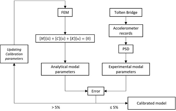
Once the numerical model has been calibrated, different types of analysis can be performed with this digital twin (Fig. 1), such as monitoring the structural health from changes in the dynamic properties or predicting the maximum stresses of the physical twin under new service conditions [13, 14]. For example, in [15, 16] a modal-observer approach was implemented in a calibrated model to estimate the time history response of all degrees of freedom of the structure, based on the acquired time histories of only some of its degrees of freedom. Then, with the information obtained, the maximum demand-capacity ratios of each element were evaluated. It is also worth highlighting the work done in [17], where Bayesian methods were implemented in a calibrated model to identify the location and magnitude of structural damage.
Fig. 1Digital twin and structural health analysis (adapted from [18])
![Digital twin and structural health analysis (adapted from [18])](https://static-01.extrica.com/articles/21246/21246-img1.jpg)
In this article, the study of structural health in a vehicular bridge that is more than 80 years old is addressed. For this purpose, a preliminary finite element model is made, based on structural drawings and visual inspections. Then, the dynamic properties of the structure are experimentally identified and with this information, the numerical model is calibrated. Finally, the digital twin of the structure is subjected to different load combinations to evaluate its behavior according to the current design standards.
2. Case study of Toltén Bridge
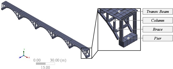
The Toltén bridge is composed of two structures, one called Original Structure (Fig. 2), built in the 1930s, and a more recent one called New Structure. The Original Structure it’s made up of ten open-arch spans, built-in reinforced concrete and with a total length of 440 meters. It has two 7.9 meters wide road lanes in each direction and two 0.8 meters wide sidewalks. The original deck consists of a reinforced concrete slab with joints between spans which lies on reinforced concrete arches attached to concrete piers. Each span is formed by two parallel arches joined by eight braces. The slab is supported by 22 columns in each span, 18 of which rest on the arches and 4 on the piers at the ends of the span. The lower part of the slab is equipped with transversal beams that join the heads of the columns two by two, giving the slab transversal stiffness.
Fig. 2Original structure
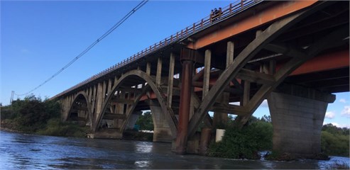
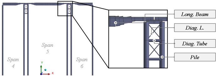
Loss of stability due to scour in pier 5 (Fig. 3), compromising the stability of spans 2 and 5, forced to perform rehabilitation works in 1993. Thus, a New Structure that consists of a concrete slab that rests on four steel girders was executed in three consecutive spans (20.8+28.6+21.2 meters) which partially replaces the Original Structure. The girders rest on circular cross-section pier columns. Two transversal struts join the heads of the piers near the Original Structure, while the eight central piers are joined by beams, forming two pier caps of four adjacent piers. In addition, under these pier caps, there is a lateral bracing formed by L-shaped and tubular profiles. The longitudinal beams are braced by L-profile trusses.
Fig. 3Scheme of the lateral view of both structures
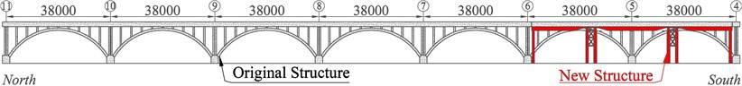
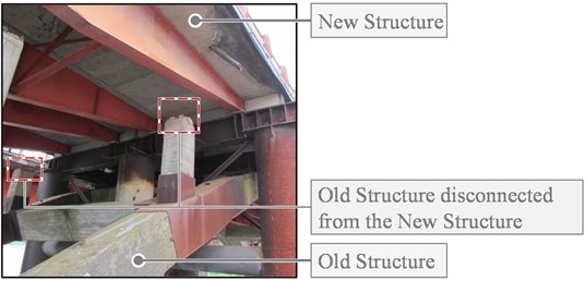
The original and New Structures do not share any element, the original substructure was disconnected from the deck in the section where the New Structure was built (Fig. 4) and there are transverse joints in the deck that disconnect the displacements between both structures. Therefore, it can be considered that the structures do not have any compatible degree of freedom, work independently, and can be modeled separately.
Fig. 4Disconnecting the original substructure (left) and disconnection between the New Structure and the original elevation (right)
According to the inspection carried out by the Ministerio de Obras Publicas of Chile in November of 2016 (Fig. 5), the bridge is in poor condition and, with the new configuration, the support of the external arches is compromised. The Bridge presents serious structural damage with burst pillars and highly undermined stocks, which may make its response unpredictable for how it was designed.
3. Finite element model
A preliminary finite element model of the original and New Structure of the Toltén Bridge was built. The model accurately represents the several element details and sizes, as it is necessary to implement a successful condition assessment of the structures [19]. Girders, beams, trusses, columns and piers were modeled as BEAM elements, suitable for slender pieces. These are 3D elements based on Timoshenko beam theory with six degrees of freedom at each node. The deck was modeled using SHELL elements, suitable for shell structures, which have four nodes with six degrees of freedom at each node. Due to the slab discontinuities between spans and it’s simply supported on abutments, displacements in slab between spans are not coupled, and only the vertical displacements between the slab and abutments are coupled. The connections between the other concrete elements are modeled completely rigid (Fig. 6).
Fig. 5Inspection of the Toltén Bridge by the Ministerio de Obras Publicas of Chile, in November of 2016
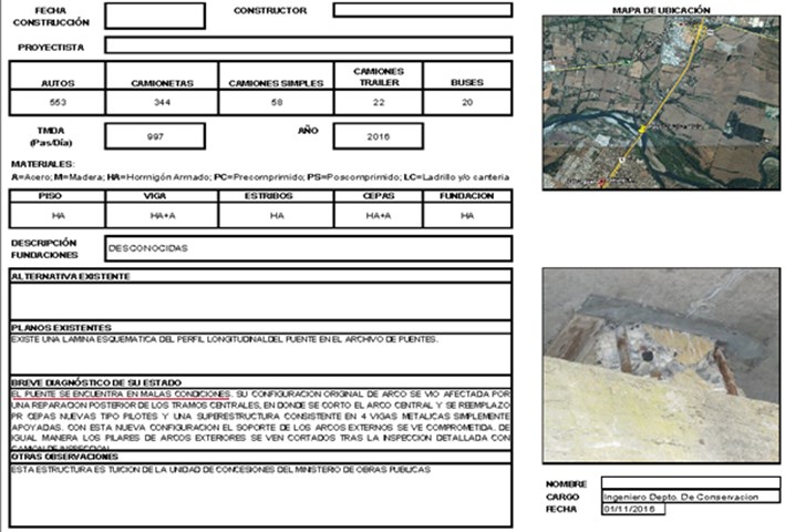
Fig. 6Finite element model of the Original Structure
The slab is also discontinuous between spans and is simply supported on the pier’s caps, so only vertical displacements between these elements are coupled. The concrete slab works in solidarity with the beams, so the 6 degrees of freedom between slab and beams have been coupled. The connections between the other elements have been modeled assuming they are completely rigid (Fig. 7 and Fig. 8).
The New Structure has a deep pier-type foundation, so it is important to establish how the stiffness of the ground varies with depth to properly reproduce the response of the ground. In this case, the ground stiffness was calculated according to the Manual de Carreteras V3, using the Eqs. (1) to (3). is the shear modulus of ground for seismic excitations in (tonf/m2), H the height of the structure buried in (m), the shear coefficient, the maximum shear coefficient, the horizontal interaction spring constant in the center of the -th layer in (tonf/m2), the distance to the center of the -th layer, measured from the roof level of the structure in (m) and the vertical effective stress in the -th pier in (tonf/m2):
With this formulation, the stiffness of the soil varies with depth and is obtained for any depth according to the stiffness on the surface. This surface stiffness is unknown and therefore will be a feature to be determined in the calibration process.
Fig. 7Finite element model of the New Structure
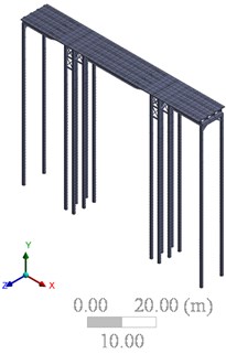
a) 3D view
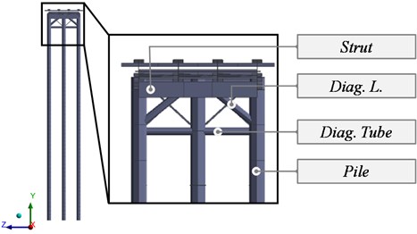
b) Front view
Fig. 8Spans 4 to 6 of the New Structure
4. Data gathering and dynamic properties identification
The use of operational modal analysis for structural health assessment has been widely studied [20-29]. This method is based on measuring the response of the structure and, through signal processing and model fitting, finding the dynamic properties that best represent the acquired signals. In this case, accelerometers were used to measure environmental vibrations in the bridge and with the identified properties the numerical model presented above was calibrated.
A modal analysis was performed on the preliminary models to verify the location of the sensors. The modal coordinates of the model were obtained in the points where the sensors would be located. It was found that, in those locations, there was not a node, at least, for the first three vibration modes. Based on this, the sensors were installed at 1/4 and 3/4 of the spans of the Original Structure, and the center of the spans of the New Structure (Fig. 9).
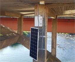
The accelerometers installed in the Original Structure are inertial sensors AltIMU-10 v5, while in the New Structure were installed unidirectional analog accelerometers MMA2241KEG. Both sensors used a sampling frequency of 100 Hz. Fig. 10 shows two sensors installed on the deck and column of the Original Structure.
Fig. 9Sensors location on structures
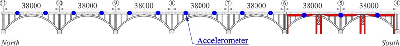
Fig. 10Sensors installed on Original Structure

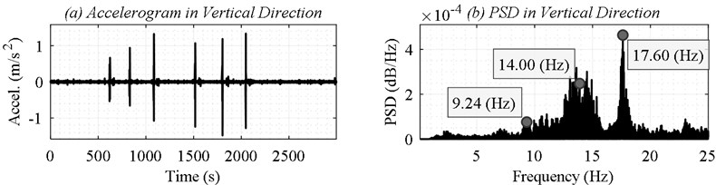
The response of Toltén Viejo (Fig. 11) and Toltén Nuevo (Fig. 12) to the passage of vehicles were measured. Subsequently, the PSDs of each accelerometer were obtained, so that the natural frequencies () of each structure (Table 1) could be determined by Peak Picking.
Fig. 11Measured response of the Original Structure in the longitudinal, transverse and vertical direction
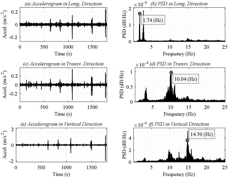
Table 1Natural frequencies identified for the Original Structure and the New Structure
(Hz) | (Hz) | (Hz) | |
Original Structure | 1.74 | 10.04 | 14.50 |
New Structure | 9.24 | 14.00 | 17.60 |
Fig. 12Measured response of the New Structure in the vertical direction
5. Model calibration
The calibration procedure is based on [30] as is detailed in Fig. 13. The approach is deployed in an iterative method which allows reducing the error within experimental and numerical results.
Fig. 13Diagram of the model calibration process
The sensitivity-based calibration method consists of three phases: (i) selection of the reference parameters, usually experimental data such as measured natural frequencies and modes of vibration, (ii) selection of the material properties to be modified, and (iii) an iterative fitting model that modifies the material properties to be updated based on the reference parameters and an objective function [31].
In Eqs. (4) and (5) it is shown that experimental reference parameters () are expressed in terms of analytical reference parameters (), structural characteristics and a sensitivity coefficient () as a first-order Taylor series [19]. is the difference between the experimental and analytical reference parameters, is the difference between the experimental structural characteristics and the estimates introduced in the model to be updated, and is the sensitivity matrix of the reference parameters with respect to the characteristics to be updated Eq. (6). and are the analytical input reference parameters and structural characteristics to be maintained:
The reference parameters used in model calibration usually include natural frequencies and eigenmodes as they can be determined from ambient vibration [20, 23, 24, 32] such as wind, earthquake and traffic. Therefore, the objective of model calibration is to minimize an objective function based on the residue between the experimental eigenfrequencies and modes and the analytical.
In this article, the reference parameters used for model calibration are the frequencies and modes of the structures themselves. The process of updating parameters and calculating errors has been implemented in MATLAB by reading the output files and modifying the script to be entered into ANSYS with the updated parameters. The geometry of the bridge, the boundary conditions and the material properties were obtained from the construction project. A visual inspection made it possible to corroborate the boundary conditions between elements as the transverse joints were operational and there was no visible damage to the connections. This is why discrepancies are associated with variation in material properties and uncertainty about boundary conditions in the field. To avoid physically meaningless results of the updated characteristics after the calibration process, upper and lower limits were determined for these values.
Because of this, the chosen material properties to be updated and their ranges of variation were:
– Density of materials. (Steel: 7-8.5 t/m3; concrete: 2.1-2.8 t/m3).
– Modulus of elasticity of the materials. (Steel: 150-220 GPa; concrete: 15-30 GPa).
– Poisson Coefficient (0.15-0.35).
– Stiffness of the terrain (30-100 MPa).
5.1. Updating the model and convergence criteria
To update the characteristics of the preliminary model, the average deviation in the fundamental frequencies was used as an objective function to be minimized, expressed as the average in the relative errors between the analytical and experimental frequencies [31]:
where is the total number of frequencies considered in the calibration, is the error between the analytical and experimental frequency and is the experimental frequency. The convergence criteria established for the iterative process were (i) value of the target function less than 5 %; (ii) minimum improvement in the target function between two iterations less than 0.1 %.
5.2. Comparison between experimental and analytical frequencies
The analytical modal parameters after the calibration process () were compared with the experimental ones () using the modal assurance criterion (MAC):
Besides, the natural frequencies of the model () and those identified by Pick Piking () were compared in terms of relative error:
MAC values above 90 % are generally accepted as an indicator of a good correlation between modes. If differences between the experimental and analytical natural frequencies are small, the calibration can be considered satisfactory [19]. In Table 2 the experimental and analytical natural frequencies area compared before and after the calibration process.
The high values of MAC along with the low errors in frequency indicate that the model can reproduce successfully the real behavior of the structure. At the beginning of this calibration process, the materials of the model were considered with typical mechanical properties, which were modified until obtaining the results shown in Table 3.
Table 2Experimental and analytical frequencies evaluation of its correlation
Before calibration | After calibration | ||||||
Original structure | |||||||
Mode | (Hz) | (Hz) | MAC (%) | Error (%) | (Hz) | MAC (%) | Error (%) |
1 | 1.74 | 1.37 | 57.60 | 21.12 | 1.67 | 92.10 | 4.02 |
2 | 10.04 | 8.47 | 83.70 | 15.69 | 10.07 | 97.70 | –0.29 |
3 | 14.50 | 12.22 | 47.10 | 15.74 | 14.39 | 95.00 | 0.76 |
New structure | |||||||
1 | 9.24 | 7.72 | 32.90 | 16.43 | 9.14 | 98.10 | 1.08 |
2 | 14.00 | 10.44 | 46.60 | 25.46 | 12.37 | 90.80 | 11.64 |
3 | 17.60 | 15.35 | 75.60 | 12.80 | 18.20 | 92.30 | –3.41 |
Table 3Initial and final material properties during the calibration process
Material properties of the model | Initial | Final |
Steel density ( / m3) | 7.80 | 7.38 |
Concrete density ( / m3) | 2.30 | 2.22 |
Modulus of elasticity of steel (MPa) | 210.00 | 202.50 |
Modulus of elasticity of concrete (MPa) | 25.00 | 27.05 |
Steel Poisson coefficient (MPa) | 0.30 | 0.28 |
Concrete Poisson coefficient (MPa) | 0.20 | 0.19 |
Stiffness of the ground on the surface (MPa) | 30.00 | 39.40 |
6. Considered scenarios
In order to find out whether the bridge complies with the regulations applicable to newly built bridges in Chile in its current state, a series of combined loads based on the regulations in force are simulated. The loads considered were traffic, wind and seismic under scouring conditions following the Highway Manual. This manual refers to the American Association of State Highway and Transportation Officials: Standard Specifications for Highway Bridges (AASHTO Standard) [33]. Methods to obtain loads from different loads as wind, scour, earthquake, and traffic are presented.
6.1. Traffic load
Traffic loads can be calculated as standard trucks or as equivalent strip loads according to AASHTO Standard. In this article, we choose to apply the HS20 standard truck [33] increasing their loads by 20 % as indicated in the Manual de Carreteras. This load has been modeled as point forces on the concrete slab.
The impact load is calculated according to the AASHTO Standard as a percentage increase of the live load using the following expression:
where is the impact fraction (maximum 30 percent) and is the length in feet of the portion of the span that is loaded to produce the maximum stress in the member. Considering the span lengths of the structures, an increase of 19 % is adopted for the Original Structure and 23 % for the New Structure.
6.2. Wind load
Wind load was considered as horizontal point loads orthogonal to the bridge’s axis equivalent to 3.6 kN/m2 on arches and frames, and 2.4 kN/m2 on beams and crossbeams as stated in the AASTHO Standard for superstructures in the transverse wind.
6.3. Earthquake scenario
The bridge’s behavior under the seismic scenario was simulated using the Response Spectrum Analysis which, for a given excitation, calculates the maximum response based on the input spectrum. Structure’s mode shapes are required to carry out the Response Spectrum Analysis, therefore the vibration mode shapes of the bridge are used from the Modal Analysis. The excitation spectrum gives absolute acceleration as a function of the natural period of the structure and the relation between accelerations and the structure’s natural frequencies. The excitation is calculated following the Manual de Carreteras formulation whose response spectrum is based on the subductive earthquake of magnitude 8.0 in the Moment Magnitude scale that took place in the central area of Chile in 1985 [34] and is calculated as follows:
where is the natural period of the mode , and are coefficients depending on the importance of the bridge and the soil, takes into account the type of soil, is the maximum effective acceleration of the ground and the threshold period. Since , the absolute acceleration can be obtained as a function of frequency as the excitation spectrum. According to the Manual de Carreteras, the Toltén Bridge is located in seismic zone 2 so it is considered a maximum acceleration of 0.3 g. The structure is considered of importance I and the soil on which it lies of type III.
The mode combination method for Response Spectrum Analysis was Square Root of Sum of Squares (SRSS) which combines the maximum values of each mode:
where is the modal response of the mode and is the total modal response.
6.4. Scour scenario
Currently, 7 meters of scour depth is reached in the piers 5 and 6 due to erosion caused by the Toltén River. Therefore, two scour scenarios were combined with each of the other loads: no scour in piers (except actual 7 meters in piers 5 and 6) and maximum scour set as the actual scour of 7 meters depth in piers 5 and 6, and also 4 meters depth in piers 2, 3 and 4. The scour has been introduced into the model by removing the springs equivalent to the different layers from the surface to the scour depth in each case, leaving the part of the foundation above the surface free.
6.5. Load combinations
The method of the admissible service loads (ASD) is adopted to check whether the bridge complies with the current standard. The formula used for the calculation of the combination of loads is that Eqs. (3-10) of the AASHTO Standard, as the Manual de Carreteras derives from this standard. Considering the loads applied to the Toltén Bridge, the following reduced formula is arrived at:
The values of and coefficients are selected for each of the AASHTO Standard load combination groups for in-service loads. According to the considered loads, and taking into account the criteria for Orthogonal Seismic Forces established in the Manual de Carreteras, the groups of loads to be calculated are those corresponding to dead and live loads, the impact of live loads, wind and earthquake (groups I, II and VII). Two directions have been considered for the earthquake: longitudinal (VIIa) and transversal (VIIb).
7. Results and discussion
The results obtained will be analyzed from two different points of view. On the one hand, it will be sought to know if the structure meets the current design criteria and, on the other hand, if its integrity can be impaired under any of the above-mentioned solicitations:
– Compliance with the current regulations, comparing the results with the admissible stresses stated in the AASHTO Standard.
– Stress limit of the material, comparing the results with the elastic limit for steel and the compressive strength for concrete.
To find out how stressed is the bridge in each of its parts, the following demand to capacity ratio is used:
where is the maximum Von Mises stress obtained by the FEM analysis and is either the maximum allowable stress set by the AASHTO Standard or for the material as mentioned in the material stress limit criterion. Therefore, a DCR value of 1 means that the limit value set by the regulations has been reached or that the capacity of the section has been exhausted. Material properties are yield strength () of 248 MPa and ultimate strength () of 20.6 MPa for structural steel and concrete respectively. By the above criteria, the permissible stresses according to the AASHTO Standard for reinforced concrete and steel are obtained ( and ).
In concrete elements subjected to bending, the stress in the most compressed fiber () must not exceed 10 MPa. Axial stresses in steel elements without gaps must not exceed 136 MPa. These stresses can be increased for some groups of load combinations according to the AASTO Standard. In Table 4 the permissible stresses are shown as a function of the load combination and the material.
Table 4Permissible stresses (ASSHTO Table 10.32.1.A and Chapter 8.15.2.1 [35])
Group | I | II | VIIa | VIIb |
Percentage | 100 % | 125 % | 133 % | 133 % |
(MPa) | 136.40 | 170.50 | 181.41 | 181.41 |
(MPa) | 8.24 | 10.30 | 10.96 | 10.96 |
7.1. Original structure
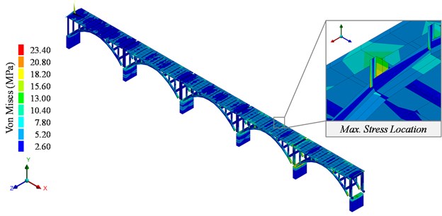
The response of the Original Structure was calculated for each load case and scour condition. For example, the maximum stress in the columns for case VIIa with the current scour is 23.40 MPa (Fig. 14). This value corresponds to a DCR of 1.14 when compared to the admissible stress of the material. A summary of each DCR for each component is presented in the following subsections.
Fig. 14Von Mises stress of the Original Structure for the earthquake in the longitudinal direction
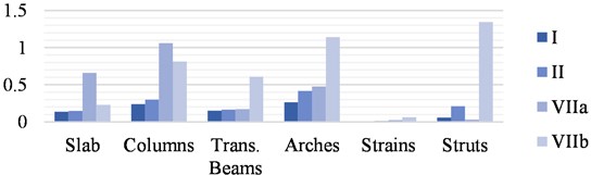
7.1.1. Compliance with current regulations
The maximum allowable stresses DCR values for each element of the Original Structure and each scenario are shown in Fig. 15 and discussed afterward.
As shown in Fig. 15, maximum stresses on the Original Structure are highly influenced by scouring values. The slab, columns and arches are the most affected elements by this scour increment, especially under traffic (I) and wind conditions (II). On the other hand, cross-beams, stumps and braces are not significantly affected by this factor. In the current situation of scouring, both the slab, columns, crossbeams, arches and braces exceed the permissible limits established by the regulations in the earthquake combination (VIIa and VIIb) while in the other combinations the values of all the elements are below the limits. In the case of maximum scour, at least two of the element types exceed the permissible limits in each combination of loads. In the combination of traffic (I) and wind (II) the limits are exceeded by the slab, columns and arches while in the longitudinal earthquake (VIIa), they are exceeded by the slab and columns. In the transverse earthquake (VIIb) only the slab and the columns do not exceed the limit values.
Fig. 15Maximum DCR for AASHTO allowable stresses in the Original Structure
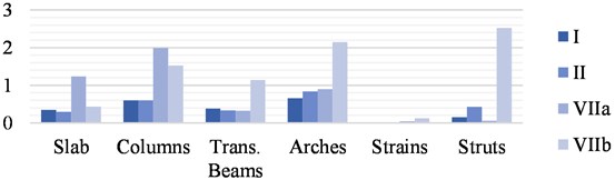
a) Current scour
b) Maximum scour
7.1.2. Stress limit of the material
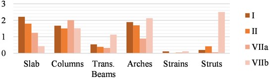
The maximum material stress limit DCR values for each element of the Original Structure and each scenario are shown in Fig. 16 and discussed afterward.
Using the strengths of steel and concrete as a reference, no element of the Original Structure exhausts its resistance capacity in the traffic load (I) and wind (II) combinations for both scour scenarios. The depletion in the load combinations with an earthquake is similar in the current scour and maximum scour scenarios, exceeding the resistance of the concrete in the columns in a longitudinal earthquake and the arches and braces in a transversal earthquake (VIIb).
The results show how the Original Structure is highly influenced by an earthquake due to the high mass of concrete, and that the stability of this structure is compromised in this case, as the concrete reaches its maximum strength in the arches which are the main supporting elements of the substructure, putting the safety of the users at risk.
Fig. 16Maximum DCR for stress limit of the material in the Original Structure
a) Current scour
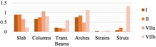
b) Maximum scour
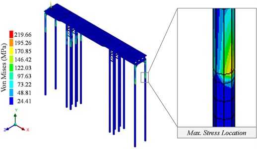
7.2. New structure
The response of the New Structure was calculated for each load case and scour condition. For example, the maximum stress in the piles for case VIIa with the current scour is 219.66 MPa (Fig. 17). This value corresponds to a DCR of 0.88 when compared to the admissible stress of the material. A summary of each DCR for each component is presented in the following subsections.
Fig. 17Von Mises stress of the New Structure for the earthquake in the longitudinal direction
7.2.1. Compliance with current regulations
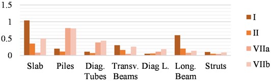
The maximum allowable stresses DCR values for each element of the New Structure and each scenario are shown in Fig. 18 and discussed afterward.
The maximum DCR values in each element type of the New Structure on each scenario are shown in Fig. 18. Scour does not affect the New Structure’s behavior as much as the original. The maximum stress in the strut is highly increased under traffic loading in the earthquake scenario. The stress increments due to scour in the rest of the elements are not significant. Under current scour values, allowable stresses are reached in the slab in traffic load case (I). Since the New Structure is slender, it is low influenced by wind load. Besides that, the allowable steel stress in the diagonal tubes is significantly increased in comparison with the current state while the stresses in the rest of the elements remain equal.
In all combinations of seismic loads, the permissible limits are reached in the piers, and only in the case of a transverse earthquake under current scour conditions are they reached in the slab. In addition, the limits at the cross-beams for the traffic combination (I) are reached in the situation of maximum scour. The values for the remaining elements are below the permissible stresses.
Fig. 18Maximum DCR for AASHTO allowable stresses in the New Structure
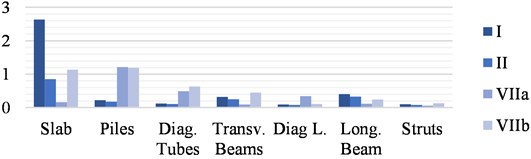
a) Current scour
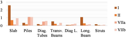
b) Maximum scour
Fig. 19Maximum DCR for stress limit of the material in the New Structure
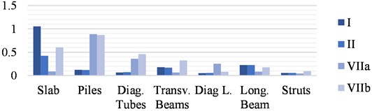
a) Current scour
b) Maximum scour
7.2.2. Stress limit of the material
The maximum material stress limit DCR values for each element of the New Structure and each scenario are shown in Fig. 19 and discussed afterward.
Using the strengths of steel and concrete as a reference, it can be seen that the stresses in the slab reach the strength of the concrete in the traffic combinations for both scour scenarios. This situation of compression breakage of the (brittle) concrete would compromise the safety of the users and leave the bridge out of service until it is repaired.
On the other hand, the New Structure behaves well in earthquakes due to the low weight-to-strength ratio of the steel, which provides a light and rigid structure and is, therefore, less susceptible to ground acceleration than massive structures.
8. Conclusions
The lack of maintenance in bridges can lead to the deterioration of their structural components, restricting the service of the structure and its capacity to resist natural events. In this article, the structural health of the Toltén Bridge has been analyzed by evaluating the capacity of its sections under different load combinations. For this purpose, a finite element model was made based on the information gathered from structural drawings and visual inspections. Subsequently, a calibration process was carried out on the model so that its dynamic properties matched with those identified experimentally. The respective load combinations were calculated, including the cases of wind, earthquake, and traffic for both scour and non-scour conditions. The maximum capacity-demand ratios (DCR) were evaluated for each component of the structure, based on the AASHTO design standards and the material capabilities. These results were analyzed, leading to the following conclusions:
1) The Original Structure does not meet the regulatory criteria in the earthquake combinations in the current scour situation or in any of the load combinations in the case of maximum scour.
2) The New Structure only meets the regulatory criteria in the wind combination under the current and maximum scour situation.
3) The New Structure behaves better in an earthquake due to the strength of steel with its mass compared to massive concrete elements, which are more influenced by ground accelerations and its foundation deep.
4) The New Structure behaves better than the original in wind due to its greater slenderness, meeting the regulatory criteria in both cases of scouring.
5) The stability of the Original Structure would be compromised in the event of an earthquake similar to that proposed by the design regulations due to the material stress limit is reached in the columns (longitudinal earthquake) or the arches (transversal earthquake), thus posing a risk to the safety of the users.
6) In the event of a traffic load as set out in the regulations, the New Structure would pose a risk to the safety of users and would be out of service due to insufficient slab capacity.
References
-
Murachi Y., Orikowski M. J., Dong X., Shinozuka M. Fragility analysis of transportation networks. in Smart Structures and Materials 2003: Smart Systems and Nondestructive Evaluation for Civil Infrastructures, Vol. 5057, 2003.
-
Deng L., Wang W., Yu Y. State-of-the-art review on the causes and mechanisms of bridge collapse. Journal of Performances od Constructed Facilities, Vol. 30, 2016, p. 2-4015005.
-
Oviedo J. A., Duque Del M. P. Seismic Response control systems in buildings. Antequio Enginering school Journal, Vol. 6, 2006, p. 105-120.
-
Reynders E. System identification methods for (operational) modal analysis: review and comparison. Archives of Computational Methods in Engineering, Vol. 19, Issue 1, 2012, p. 51-124.
-
Saridis G., Stein G. Stochastic approximation algorithms for linear discrete-time system identification. IEEE Transaction Automatatic Control, Vol. 13, Issue 5, 1968, p. 515-523.
-
Van Overschee P., De Moor B. N4SID: Subspace algorithms for the identification of combined deterministic-stochastic systems. Automatica, Vol. 30, Issue 1, 1994, p. 75-93.
-
Chang M., Pakzad S. N. Modified natural excitation technique for stochastic modal identification. Journal of Structural Engineering, Vol. 139, Issue 10, 2013, p. 1753-1762.
-
Van Overschee P., De Moor B. Subspace Identification for Linear Systems. Springer, Boston, 1996.
-
Peeters B., De Roeck G. Stochastic System Identification for operational modal analysis: a review. Journal of Dynamic Systems Measurement Control, Vol. 123, Issue 4, 2001, p. 659-667.
-
Diez A., Khoa N. L. D., Makki Alamdari M., Wang Y., Chen F., Runcie P. A clustering approach for structural health monitoring on bridges. Journal of Civil Structures Health Monitoring, Vol. 6, Issue 3, 2016, p. 429-445.
-
Sevim B., Bayraktar A., Altunişik A. C., Atamtürktür S., Birinci F. Finite element model calibration effects on the earthquake response of masonry arch bridges. Finite Element Analysis Design, Vol. 47, Issue 7, 2011, p. 621-634.
-
Zhang Q. W., Chang T. Y. P., Chang C. C. Finite-element model updating for the Kap Shui Mun cable-stayed bridge. Journal Bridge Engineering, Vol. 6, Issue 4, 2001, p. 285-293.
-
Orlowitz E., Brandt A. Comparison of experimental and operational modal analysis on a laboratory test plate. Measurement, Vol. 102, 2017, p. 121-130.
-
Tuegel E. J., Ingraffea A. R., Eason T. G., Spottswood S. M. Reengineering aircraft structural life prediction using a digital twin. International Journal Aerospatial Engineering, Vol. 2011, 2011, p. 154798.
-
Hernandez E., Roohi M., Rosowsky D. Estimation of element-by-element demand-to-capacity ratios in instrumented SMRF buildings using measured seismic response. Earthquake Engineering Structural Dynamics, Vol. 47, Issue 12, 2018, p. 2561-2578.
-
Roohi M., Erazo K., Rosowsky D., Hernandez E. M. An extended model-based observer for state estimation in nonlinear hysteretic structural systems. Mechanical Systems Signal Processing, Vol. 146, 2021, p. 107015.
-
Behmanesh I., Moaveni B. Probabilistic identification of simulated damage on the Dowling Hall footbridge through Bayesian finite element model updating. Structural Control Health Monitoring, Vol. 22, Issue 3, 2015, p. 463-483.
-
Muñoz E., Nunez F., Rodríguez J. A., Ramos A., Otálora C. Seismic vulnerability and load capacity of a cable-stayed bridge based on structural reliability. Construction Engineering Journal, Vol. 25, Issue 2, 2010, p. 285-323.
-
Brownjohn J. M. W., Xia P. Q., Hao H., Xia Y. Civil structure condition assessment by FE model updating: methodology and case studies. Finite Element Analysis Design, Vol. 37, Issue 10, 2001, p. 761-775.
-
Brownjohn J. M. W., Magalhaes F., Caetano E., Cunha A. Ambient vibration re-testing and operational modal analysis of the Humber Bridge. Engineering Structures, Vol. 32, Issue 8, 2010, p. 2003-2018.
-
Brownjohn J. M. W., Moyo P., Omenzetter P., Lu Y. Assessment of highway bridge upgrading by dynamic testing and finite-element model updating. Journal of Bridge Engineering, Vol. 8, Issue 3, 2003, https://doi.org/10.1061/(ASCE)1084-0702(2003)8:3(162).
-
Butt F., Omenzetter P. Seismic response trends evaluation and finite element model calibration of an instrumented RC building considering soil-structure interaction and non-structural components. Engineering Structures, Vol. 65, 2014, p. 111-123.
-
Wu J. R., Li Q. S. Finite element model updating for a high-rise structure based on ambient vibration measurements. Engineering Structures, Vol. 26, Issue 7, 2004, p. 979-990.
-
Bayraktar A., Birinci F., Altunışık A. C., Türker T., Sevim B. Finite element model updating of senyuva historical arch bridge using ambient vibration tests. Journal of Road Bridge Engineering, Vol. 4, Issue 4, 2009, p. 177-185.
-
Stavroulaki M. E., Riveiro B., Drosopoulos G. A., Solla M., Koutsianitis P., Stavroulakis G. E. Modelling and strength evaluation of masonry bridges using terrestrial photogrammetry and finite elements. Advances in Engineering Software, Vol. 101, 2016, p. 136-148.
-
Zampieri P., Zanini M. A., Faleschini F., Hofer L., Pellegrino C. Failure analysis of masonry arch bridges subject to local pier scour. Enginering of Failure Analysis, Vol. 79, 2017, p. 371-384.
-
Malm R., Andersson A. Field testing and simulation of dynamic properties of a tied arch railway bridge. Engineering Structures, Vol. 28, Issue 1, 2006, p. 143-152.
-
Chung W., Sotelino E. D. Three-dimensional finite element modeling of composite girder bridges. Engineering Structures, Vol. 28, Issue 1, 2006, p. 63-71.
-
Hong A. L., Ubertini F., Betti R. Wind analysis of a suspension bridge: Identification and finite-element model simulation. Journal of Structural Engineering, Vol. 137, Issue 1, 2011, https://doi.org/10.1061/(ASCE)ST.1943-541X.0000279.
-
Friswell M., Mottershead J. E. Finite element model updating in structural dynamics. Springer Science and Business Media, Vol. 38, 2013.
-
Butt F., Omenzetter P. Finite element model calibration of an instrumented RC building based on seismic excitation including non-structural components and soil-structure-interaction. 22nd Australasian Conference on the Mechanics of Structures and Materials, 2013, p. 251-256.
-
Chen X., Omenzetter P., Beskhyroun S. Calibration of the finite element model of a twelve-span prestressed concrete bridge using ambient vibration data. 7th European Workshop on Structural Health Monitoring, 2nd European Conference of the Prognostics and Health Management (PHM) Society, 2014.
-
Dakota N. American Association of State Highway and Transportation Officials, 2010.
-
Instruction and Design criteria. Roads Construction Ministery, Vol. 1, 2008.
-
Aashto L. Standard specifications for highway bridges. 17th Edition, American Association State Highwai Transportation of Washington, DC, 2002.
About this article

