Abstract
In this paper, mathematical model of Monkey-Pox transmission is developed and investigated, using ordinary differential equation. We verified the feasible region of the model and showed the positivity of the solutions. We obtained the disease free equilibrium (DFE). We computed and analysed the effective basic reproduction number () of the model.
Highlights
- The study found the disease free equilibrium and effective reproduction number of the model equations
- Epidemiological implication is that if the secondary cases of the monkey pox infection and human cases are on average less than one unit, then the disease will die out on the long run
- The study incorporated exposure and vaccination class
- The monkey pox will be eradicated among human population, provided R_h >1
1. Introduction
Monkey-pox is known as pathogens, affecting livestock animals and humans and belongs to the orthopox virus, which included small pox cause infection in humans and cow pox viruses [1]. The monkey pox causes lymph nodes to swell. The symptoms are fever, headache, muscle aches, backache, swollen lymph nodes, a feeling of discomfort and exhaustion. The virus is similar to small pox in human. The virus can spread both from animal to human and from human to human. The increased transmission risk associated with factors involving introduction of virus to the oral mucosa [2].
The incubation period range from 7 to 14 days. After 1 to 3 days of the appearance of fever, the patient develops raised bumps and the illness lasted for 2 to 4 weeks [5]. Thus, the reported case fatality ratio is range from 1 % to 10 % [3]. Currently, there are no vaccines for monkey pox, however, evidence showed that small pox vaccine reduced the risk of monkey pox among previously vaccinated persons in Africa [4, 5]. Centre for disease control and prevention also recommended that persons investigating monkey pox outbreaks and caring for infected individuals should vaccinated with small pox vaccine, to protect against the monkey pox. Individuals who have had close contact with persons confirmed to have monkey pox should be vaccinated up to 14 days after exposure were recommended [4].
Mathematical models have played a central role to capture the dynamics of different Disease transmission [6]. The aim of this paper is therefore to the development and exploration of a mathematical model for transmission of monkey-pox disease in humans. Therefore, there is non-numerous work on mathematical modelling of monkey pox transmission. This Paper extends the work of [7] by incorporating Vaccination class for migrants, Exposed classes for both human and non-human population.
2. Model formulation
We formulate a model for the spread of Monkey-pox in human and primates (Monkey) population with the total population size at time t given by and . The populations are further compartmentalized into epidemiological classes as shown in the model flow diagram in Fig. 1. The total human population is divided into five subgroups that is the Susceptible, , the Vaccinated, , the Exposed, , the Infected, , and the Recovery with permanent immunity, . The total primates (Monkey) population model divides into the Susceptible, , the Infected primates, , the Exposed, and the recovery with permanent immunity, . As indicated in the compartmental diagram in Fig. 1, people enter Susceptible class through birth and immigration, (), where a proportion of vaccinated human immigrants () enter to the vaccinated class and proportion of unvaccinated immigrants () enter to the susceptible class. We do not consider the immigration of infection person, because we assume that people who are coming from monkey-pox endemic zones have to be vaccinated. The susceptible individuals vaccinated at the rate and loss the vaccination at the rate . Susceptible human get contact from primate at rate , are exposed to monkey-pox infection at the rate and infected at the rate , with natural death and die due to the infection at the rate and recovery with permanent immunity at a rate . The Susceptible primates, class is generated from the daily recruitment of individuals through birth and immigration at the and natural death rate . They become exposed to monkey-pox virus at the rate and leave the class to infected class at the rate . Individuals primate infected die due to the infection at the rate and recovery with the permanent immunity at the rate .
Fig. 1Schematic diagram of transmission of monkey-pox disease
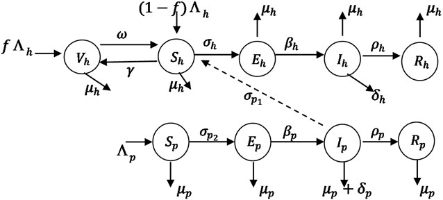
Base on the above assumptions and schematic diagram of Fig. 1, the model for transmission dynamics of Monkey-pox infection in human and primates (Monkey) is described by a system of Ordinary Differential Equations (ODEs) given below:
where:
The susceptible human host get infected from both the infected primate () and infected human () which is called force of infection from primates to human as well as human to human [7]. The term is the product of the effective contact rate and probability of the human being get infected from the infected primates () and is the product of the effective contact and probability of the human get infected from the infected persons (). Similarly, the get infected from infected primate, where is the product of the effective contact rate and probability of the primates (monkey) get infected per contact with an infected primate () [7]. The modification parameter account for the assumption that exposed human transmits at a rate lower than symptomatic humans. The modification parameter account for the assumption that exposed non-human transmits at a rate lower than symptomatic non-humans. It is assumed here that mortality of monkeys due to being hunted by humans is negligible and can be safely ignored.
3. Analysis of the model equations
Theorem 1: (Invariant Region) the following biological feasible region of the model Eqs. (1)-(9) , : is positively invariant and attracting.
Proof; the addition of all the equations model in Eqs. (1)-(9) give:
So that:
It follows from [8], the Gronwall inequality, that:
In particular, if and if . Thus, is positively invariant. Hence, it is sufficient to consider the model dynamics Eqs. (1)-(9) in , in this region, the model equations can be considered as been epidemiologically and mathematically well posed.
Theorem 2: (Positivity of the Solution for the Model). Let and the initial conditions satisfied , , , , , , 0, 0, , then the solutions , , , , , , , , , of the model Eqs. (1)-(9) are positive for all .
Proof:
Proving that for all , , , , , , , , , will be positive in , Since all the parameters used in the system are positive. Thus, it is clear from Eq. (1) that:
So that:
The similar approach can be used to show that , , , , , 0, 0, . Thus, for all , , , , , , , , , will be positive and remain in .
4. Existence of the equilibrium
At equilibrium state, we let:
From Eq. (3), we have:
Substitute Eq. (16) into Eq. (2), we have:
Equation (17) gives:
From Eq. (8), we have:
Substitute Eq. (19) into Eqs. (7), we have:
Equation Eq. (20) gives:
Substitute in Eq. (9) into Eq. (16) and Eq. (5), we have:
Making subject of expression in Eq. (4) and Eq. (1), and equating them, we have:
Implies:
Since , implies , then we have:
Reduced to:
If there is no vaccination, then as .
Substitute Eq. (25) into Eq. (4), we have:
Substitute in Eq. (21) into Eqs. (19) and (9), we have:
From Eq. (6), we have:
The disease free equilibrium (DFE) state is given as:
5. Effective basic reproduction number ()
We applying next generation matrix operator to compute the effective basic reproduction number [9]. The largest Eigenvalue or spectral radius of is the effective basic reproduction number of the model:
where is the rate of appearance of new infection in compartment , is the transfer of infection from one compartment to another and is the Disease-Free Equilibrium.
Using this technique, we have spectral radius () of the next generation matrix, that is, . Both and are obtained from the Jacobian matrix of the linearization of system Eqs. (1)-(9) disease free equilibrium. Therefore, the vector and representing inflow and outflow from compartments , , and are given by:
where, ; ; ; and:
From Eqs. (34), we have:
At DFE, and since and we have:
From Eq. (36), we have:
Multiplying Eq. (37) and (35) together, we have:
Equation (39) implies:
The characteristics equation of Eq. (40), gives :
where:
Determinant of Eq. (41) gives:
To solve Eq. (43) with completing the square method, we have:
is the spectral radius of and the reproduction number is the largest eigenvalue from Eq. (44):
Implies:
is the spectral radius of :
Then, we obtained effective basic reproduction number as Eqs. (48) and (45). There are two host populations and it was shown from the model flow diagram in Fig. 1 that the monkey transmits the infection to human host and human to human. Hence, the effective basic reproduction number can be represented as:
5.1. Analysis of effective basic reproduction number on and
Form Eq. (45), we have:
where:
Since the disease will not be established in the population if the secondary cases on average is less than a unit (), this implies:
From Eqs. (53), we have:
Implies:
From Eqs. (55), we make the product of the effective contact rate and probability of the primates (monkey) get infected per contact with an infected primate as a subject, we have:
Where:
Also, we make the infected at the rate as a subject:
Where:
In a similar case, since the disease will not be established in the population if the secondary case on average is less than a unit ().
Form Eq. (48), we have:
where:
From Eqs. (65), we have:
Implies:
From Eqs. (67), we make the product of the effective contact and probability of the human get infected from the infected persons as a subject, we have:
where:
Also, we make the infected at the rate as a subject:
where:
6. Conclusions
The Monkey pox will be eradicated since the term is greater than the product of the effective contact rate and probability of the primates (monkey) getting infected and the term is greater than infected rate as shown in Eq. (60), provided . However, since , it means that there is no transmission between primates and humans population at disease free equilibrium. Similarly, the monkey pox will be eradicated among human population, since the term is greater than and is greater than as shown in Eq. (72), provided . Epidemiological implication is that if the secondary cases of the monkey pox infection and human cases are on average less than one unit, then the disease will die out on the long run.
In this paper, we developed a mathematical model of monkey-pox transmission disease. We analysed the invariant region and shown that the dynamics of model Eqs. (1)-(9) is in the region , the model equations was considered as been epidemiologically and mathematically well posed. The positivity of the solutions for the model was showed which implies that the solutions were positive and remains in . The disease free equilibrium and effective basic reproduction number of the model were obtained. Analyses of effective basic reproduction number were done.
References
-
Essbauer S., Pfeffer M., Meyer H. Zoonotic poxviruses. Veterinary Microbiology, Vol. 140, Issues 3-4, 2010, p. 229-236.
-
Kantele A., Chickering K., Vapalahti O., et al. Emerging diseases – the monkey pox epidemic in the Democratic Republic of the Congo. Clinical Microbiology and Infection, Vol. 22, Issue 8, 2016, p. 658-659.
-
Rimoin A. W., Kisalu N., Kebela Ilungam B., et al. Endemic human monkey pox, Democratic Republic of Congo, 2001-2004. Emerging Infectious Diseases, Vol. 13, Issue 6, 2007, p. 934-936.
-
Centres for Disease Control Morbidity and Mortality Weekly Report. Atlanta, Georgia (MMWR), Vol. 52, Issue 27, 2003, p. 642-646.
-
What You Should Know About Monkeypox. Fact Sheet. Centres for Disease Control and Prevention, 2003.
-
Lasisi N. O., Akinwande N. I., Olayiwola R. O., et al. Mathematical model for Ebola virus infection in human with effectiveness of drug usage. Journal of Applied Sciences and Environmental Management, Vol. 22, Issue 7, 2018, p. 1089-1095.
-
Bhunu C. P., Mushayabase S. Modelling the transmission dynamics of pox-like infections. International Journal of Applied Mathematics, Vol. 41, Issue 1, 2011, p. 2-9.
-
Bauch C., Earn D. Transients and attractors in epidemics. Proceedings of the Royal Society of London Series A, Vol. 270, Issue 1, 2003, p. 1573-1578.
-
Van den Driessche P., Watmough J. Reproduction numbers and sub threshold endemic equilibria for the compartmental models of disease transmission. Mathematical Biosciences, Vol. 180, Issue 1, 2002, p. 29-48.
Cited by
About this article

