A road quality classification technique based on vehicle system responses with experimental validation

Dang, Xiaozheng; Zhou, Liangsheng; Wei, Xiaojun; Wang, Yushuai

doi:10.21595/jve.2020.21222

Journal of Vibroengineering

Browse Journal

Submit article

Published: 30 September 2020

Check for updates

A road quality classification technique based on vehicle system responses with experimental validation

Xiaozheng Dang¹

Liangsheng Zhou²

Xiaojun Wei³

Yushuai Wang⁴

^{1, 2, 3}Military Traffic and Transpotation Institute, Military Transportation University, Tianjin, Tianjin, China

⁴College of Mechatronics Engineering, North University of China, Tianjin, Tianjin, China

Corresponding Author:

Yushuai Wang

Cite the article Download PDF

Downloads 793

WoS Core Citations 1

CrossRef Citations 1

Abstract

Aiming at estimating the road surface condition with improvement of the accuracy in spatial, this paper proposes a new method to classify road surface condition by considering identification interval based on vehicle system responses. First, the response signals in different vehicle speeds are decomposed by using both Wavelet Transform (WT) and Empirical Mode Decomposition (EMD) techniques. Then characteristics of the signals in both the time and decomposed frequency domain are subsequently extracted. An Improved Distance Evaluation Technique (IDET) is used to select superior features from the characteristics. Finally, a Support Vector Machine (SVM) classifier is applied to determine the road classification. The influences of identification intervals in spatial accuracy are discussed, and an adaptive classification interval was proposed to improve accuracy. The algorithm is validated by using both simulation and experimental results.

A road quality classification technique based on vehicle system responses with experimental validation

Highlights

A combined Wavelet Transform (WT) and Empirical Mode Decomposition (EMD) method to process the measured signals is developed.
Vehicle speed is determined to be an important feature in successful classification.
The identification interval is constrained by a compromise between analysis accuracy and sufficient information.

1. Introduction

Road roughness is used to describe roadway serviceability and has been one of the widely accepted criteria for road conditions assessment to guide maintenance planning. Quality of road roughness will dramatically affect vehicle wear, ride quality, and transportation safety. The large dynamic axle loading from roughness accelerates pavement deterioration, so pavement engineers have to maintenance the road in relatively good level all the time [1]. However, analysis and measurement of road roughness is a difficult problem that pavement engineers have been facing for many years, especially the road which heavy vehicles such as truck often make lots of stop-and-go trips [1]. Detection and maintenance of the condition of a road profile is important for many reasons, such as safety and economic savings. In this case, road roughness detection and maintenance become one of the most concerns of road engineers.

Current road estimation methods can be divided into three categories [2], namely, direct measurements [3, 4], non-contact measurements [5] and system response based estimation [6-12]. Among these three categories, the first two require specific instruments designs, which restrict their practical applications. Depending on sensors that were originally designed for system control, the last method is often used to estimate road excitation. The use of vehicle system response to estimate road condition have been investigated some years, and the applications take advantage of the technique to control vehicle height [13], change suspension parameters [14, 15] and guide maintenance planning of road engineers.

The aim of this paper is to develop a new method of estimating the general conditions of road by using the response signals of vehicle, with experimental validation. Appropriate and measurable signals are firstly sampled. A combined Wavelet Transform (WT) [16, 17] and Empirical Mode Decomposition (EMD) [18] analysis is then performed to the sampled signals and the candidate decomposed signals are obtained. Four statistical measures, namely: Variance (Var); Square Root of Amplitude (SRA); Root Mean Square (RMS); and Maximum value (Max.), are used to characterize the candidate signals. Dimensionality issues are avoided by selecting the most dominant characteristics using an Improved Distance Evaluation Technique (IDET). Finally, a Support Vector Machine (SVM) classifier is applied to the output to classify the road.

The novel contributions of this research are as follows:

– Novel combination of signals processing method.

From the requirement of minimizing the effects of measurement noise, this paper developed a combined WT and EMD method to process the measured signals. It takes full advantage of both the WT and EMD techniques and improves the estimation accuracy.

– Investigation of speed influence.

Different traffic conditions may lead to various vehicle speeds. As such vehicle speed is an important factor that should be taken into consideration. Vehicle speed is determined to be an important feature in successful classification.

– Investigation of identification interval.

Shorter identification intervals come with shorter road length identification intervals and higher accuracy of the road surface analysis, but it’s hard to obtain sufficient information on low frequency components signal if interval is too short. Thus, the interval is constrained by a compromise between analysis accuracy and sufficient information to enable identification. Considering the variation in vehicle speed, the adaptive interval with variation speed is first proposed to improve road surface analysis accuracy in spatial.

The structure of the paper is as follows: in Section 2, the vehicle and road models are introduced; then in Section 3, the definition of superior features in both the time and frequency domain are provided; Section 4 introduces the structure of the proposed method, including signal pre-processing, feature reduction and classification with SVM; the results of the simulations and experiments used for validation are discussed in Section 5 and Section 6 respectively; finally, conclusions are drawn in Section 7.

2. System models

2.1. Vehicle model

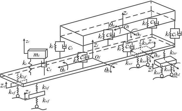
A thirteen Degree of Freedom (DOF) truck model which considers the heave-pitch-roll motions of various sections is introduced, as shown in Fig. 1.

Fig. 1Full-scale truck model

The dynamic equations of the model are given by Eq. (1):

1

M \ddot{X} + C \dot{X} + K X = F X_{r},

where $M$ , $C$ , $K$ and $F$ are the mass matrix, damping matrix, stiffness matrix and coefficient matrix of the road input respectively, (see Appendix). $X_{r}$ is road input of six wheel (more details in Section 1.2). Define the state vector $X$ as:

X = {[\begin{array}{l} z_{l f} & z_{r f} & z_{l r} & z_{r r} & θ_{l s l} & θ_{l s r} & z_{f} & θ_{f x} & θ_{f y} & z_{c} & z_{t} & θ_{t x} & θ_{t y} \end{array}]}^{T},

where $z_{l f}$ , $z_{r f}$ , $z_{l r}$ , $z_{r r}$ , $z_{f}$ , $z_{c}$ and $z_{t}$ are the left front unsprung mass displacement, right front unsprung mass displacement left rear unsprung mass displacement, right rear unsprung mass displacement, frame mass displacement and compartment mass displacement, respectively. Similarly $θ_{l s l}$ , $θ_{l s r}$ , $θ_{f x}$ , $θ_{f y}$ , $θ_{t x}$ and $θ_{t y}$ are the roll angle of the left rear unsprung mass, roll angle of the right rear unsprung mass, roll angle of the frame, pitch angle of the frame, roll angle of the compartment and pitch of the compartment, respectively.

2.2. Road model

2.2.1. Road irregularities

The distance between the road surface and base plate is typically defined as the function of road irregularities $q (I)$ . Often, the road profile is assumed to be homogeneous and with a Gaussian random process. As such its statistical characteristics can be described by a Power Spectral Density (PSD) [5]. This paper establishes the road surface model in accordance to the international standard ISO 8608 [19], and the PSD of the road roughness can be approximated by Eq. (2):

2

G_{q} (n) = G_{q} (n_{0}) {(\frac{n}{n_{0}})}^{- W},

where, $n$ is the spatial frequency in m^-1, indicates the number of wavelength in per meter, and $n_{0}$ is the reference spatial frequency with the value of 0.1 m^-1. $G_{q} (n_{0})$ is the PSD in the reference spatial frequency in m³ and $W$ is called the waviness, which reflects the approximate frequency structure for a certain range of road profile. Reference [7] reveals that the value of $W$ varies from 1.6-2.4 with mean value of 2, to 1.5-3.5 with mean value of 2.5, recorded over the past 30 years. It is assumed that $W =$ 2 in this paper.

When a vehicle is driving with a velocity $v$ , the spatial frequency $n$ in Eq. (2) can be transformed into a time frequency $f$ according to Eq. (3):

3

f = v n,

where $f$ is the time frequency in Hz.

In order to ensure the accuracy of the road estimation and comprehensiveness of vehicle system response, the range of wavelengths needed to be defined carefully. According to ISO8608, the spatial frequency range is commonly assumed to be 0.011 m^-1-2.83 m^-1 for in-road vehicles. This ensures that under the commonly used vehicle speed of 36-108 km/h, the range of time frequency covers 0.33 Hz-28.3 Hz. The pitch natural frequency of 0.5-1 Hz, the sprung mass natural frequency of 1-2 Hz and the unsprung mass natural frequency of 10-15 Hz are included in this range, so that the vehicle dynamic response can be reflected accordingly.

2.2.2. Road characteristics in the transverse direction

The correlations in the excitations of the left and right path are described by the coherence of the excitations [8, 9, 20-22]:

4

γ (ρ, n) = \frac{G_{l r} (n)}{\sqrt{G_{l l} (n) G_{r r} (n)}},

where the indices $l$ and $r$ denote the left and right path of the vehicle respectively and $ρ$ is the track width.

2.2.3. Road high profile modeling

Two different approaches are widely discussed in the literature for modeling road irregularities:

– Synthesis using harmonic functions and randomly distributed phases [10].

– Synthesis based on noise-excited linear dynamic systems [11].

A road excitation process with waviness $w =$ 2 can be generated by means of a simple first-order filter:

5

\dot{ξ} + ω ξ = \sqrt{v G_{0} n_{0}^{2}} z, z = z (k Δ t) = \sqrt{\frac{12}{Δ t}} Z_{k}, k = 0,1, 2, . . .,

where $Z_{k}$ is a random number sequence in the range of [–0.5, 0.5], which is called up in sufficiently small time intervals $∆ t$ . The road excitation $ξ$ approximates the desired target spectrum for frequencies above $f > w_{g} / 2 p$ with intensity $G_{0}$ and waviness $W =$ 2.

2.2.4. Two-track excitations

Two-track road excitations, with coherence characteristics close to reality, are generated through a straightforward mixing function. Two independent excitations $ξ_{1}$ and $ξ_{2}$ are used as input signals which have already been adjusted to the desired longitudinal direction spectrum. From these signals, two coupling signals $η_{1}$ and $η_{2}$ are generated through first-order filters:

6

{\dot{η}}_{1} + n η_{1} = n ξ_{1}, {\dot{η}}_{2} + n η_{2} = n ξ_{2} .

Thereby, with the original excitations $ξ_{1}$ , $ξ_{2}$ the desired road excitations $q_{l} (I)$ , $q_{r} (I)$ are generated [21]:

7

q_{l} (I) = ξ_{1} - (1 - \frac{\sqrt{2}}{2}) η_{1} + \frac{\sqrt{2}}{2} η_{2}, q_{r} (I) = ξ_{2} - (1 - \frac{\sqrt{2}}{2}) η_{2} + \frac{\sqrt{2}}{2} η_{1},

where $q_{l} (I)$ , $q_{r} (I)$ are left track and right track of wheels, respectively. Assuming that vehicle is running straight line, road inputs of six wheels are obtained:

8

X_{r} = [\begin{array}{l} q_{l} (I) & q_{r} (I) & q_{l} (I + l_{1}) & q_{l} (I + l_{2}) & q_{r} (I + l_{1}) & q_{r} (I + l_{2}) \end{array}],

where, $l_{1}$ is displacement of front-wheels and middle-wheels, $l_{2}$ is displacement of front-wheels and rear-wheels, respectively.

3. Feature definition

Qin et al. [2] has proposed, in total, 11 different features for salient selection. Their results reveal that features related to signal energy perform much better than other categories. In this paper, Var, SRA, RMS and Max. of the signals are chosen as basic statistical features. For a signal $x (n)$ of length $N$ , the definitions of the above four features are as follows:

9

V a r i a n c e = \sqrt{\frac{\sum_{n = 1}^{N} {(x (n) - \bar{x})}^{2}}{N - 1}} ， S R A = {(\frac{\sum_{n = 1}^{N} \sqrt{|x (n)|}}{N})}^{2},

R M S = \sqrt{\frac{\sum_{n = 1}^{N} {(x (n))}^{2}}{N}} ， M a x = m a x |x (n)|,

where $\bar{x}$ is the mean value of $x (n)$ .

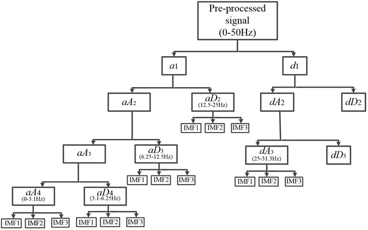
Since the road excitation frequency is related to vehicle velocity, it has a relatively small amplitude in low velocity systems and a large amplitude in high velocity systems. The generated responses of each of these systems are quite different and so the system response of different frequency ranges should be fully investigated. Qin [23] proposed an effective method to decompose vehicle system responses by using wavelet analysis, taking advantage of its strong ability of processing noisy signals. However, wavelet transform performance is largely depended on the wavelet basis functions and signal processing results are different using different wavelet basis. To avoid this, a combined treatment method of wavelet analysis and Empirical Mode Decomposition (EMD) is utilized to process the vehicle signals. EMD is a method for decomposing nonlinear, multicomponent signals. The components resulting from EMD, called Intrinsic Mode Functions (IMF), each admit an unambiguous definition of instantaneous frequency and amplitude. However, EMD can be subject to aliasing effects when the signal changes rapidly. The method used in this paper can be described as: using the wavelet transforms to decompose the signal into narrow-banded signals, then using EMD to decompose these narrow-banded signals. The structure of the decomposition is shown in Fig. 2.

Fig. 2Structure of the combined WT and EMD decomposition technique

Including both time and frequency information, 64 features are calculated in total based on the four statistical metrics in Eq. (9). These features are stated as follows:

– 4 measured signal features: the four basic statistical quantities of the measured signal.

– 60 decomposed signal features: five different frequency range signals are generated by the wavelet transform, corresponding to the range 0.8-31.3 Hz; then 15 IMF signals are obtained by getting first three IMF of one frequency range signal using the EMD technique. Then 60 features are calculated based on the four statistical quantities of each IMF.

4. Classification algorithm

4.1. Signal sampling and pre-processing

In order to correctly extract features from the measured signals and improve the accuracy of the classification, some pre-processing is firstly performed. The pre-processing includes three steps, namely: low pass filtering; framing; and windowing.

– Low-pass filtering.

To avoid signal aliasing, a low pass filter with a cut-off frequency of 50 Hz is firstly applied, as the sampling rate and the upper frequency bound are set to be 100 Hz and 31.3 Hz respectively.

– Framing.

The classification interval is assumed to be fixed 1 second. Larger intervals may deteriorate its performance by data redundancy and it is hard to achieve high resolution for low frequency components if a smaller interval is chosen.

– Windowing.

To prevent spectral leakage at the beginning and end of a frame, a Hamming window of the following form is applied:

10

W (k) = 0.54 - 0.46 c o s (2 π \frac{k}{N - 1}), k = 0,1, . . . N - 1,

where $N =$ 200 is the number of points of each frame. Assuming $x (t)$ to be the signal in a frame, the output signal, $y (t)$ , after windowing can be expressed as:

11

y (t) = x (t) \times w (t) .

It should be noted that this pre-processing procedure is indispensable for both classifier training and the validation process.

4.2. Feature reduction

After feature fusion, 64 features are obtained in total. It is possible to use all of these features to perform the classifier; however, two restrictions may deteriorate its performance:

– Dimensionality.

Since the complexity of the SVM classifier is largely depending on the dimensions of the input variables, the large number of input variables in this case may lead to a significant incense in computation time.

– Data redundancy.

Combining all individual good features may not always result in superior classification performance. The truth is under the premise of accuracy, if fewer features are used, the method is better. In this situation, the method to select features with minimal redundancy is required.

To solve the aforementioned problems, a suitable method to select superior features is needed. Here, an Improved Distance Evaluation Technique (IDET) was applied to select the maximal relevance features [23, 24]. The improved distance evaluation procedure is described as follows:

Suppose a road feature set with $C_{r}$ levels and $J$ features can be described as:

12

\{q_{m, j, c}, m = 1,2, \dots M_{r}, j = 1,2, \dots J, c = 1,2, \dots C_{r},\},

where $q_{m, j, c}$ is the $m$ th sample of the $j$ th feature belonging to the $c$ th level. $M_{r}$ and $J$ are the total number of samples and features, respectively. The distance evaluation procedure can be depicted in Table 1.

Features with higher ${\bar{α}}_{j}$ can be interpreted as the sample distance of all levels which are more obvious than others. They can be applied to improve separation among different levels. Some features are then collected to form a set of superior features and can be further used in the formulation of the classifier. The value of $M_{r}$ , $J$ , $C_{r}$ and the superior feature set are defined as follows: $M_{r} =$ 100 for each level in the classifier training process, corresponding to the training and testing samples; the number of features $J =$ 64; and the number of road excitation levels $C_{r} =$ 32.

Table 1The improved distance evaluation procedure

a) Calculate the sample variance factor:

v_{j}^{(w)}

v_{j}^{(w)} = \frac{m a x (d_{j, c})}{m i n (d_{j, c})}

, where

d_{j, c} = \frac{2 \times \sum_{k, l}^{M_{r}} |q_{k, j, c} - q_{l, j, c}|}{M_{r} \times (M_{r} - 1)}

,

k, l = 1,2, \dots M_{r}

,

k \neq l .

b) Calculate the level variance factor:

v_{j}^{(b)}

v_{j}^{(b)} = \frac{m a x (|u_{j, p} - u_{j, q}|)}{m i n (|u_{j, p} - u_{j, q}|)}

, where

u_{j, c} = \frac{\sum_{m = 1}^{M_{r}} q_{m, j, c}}{M_{r}} .

c) Calculate the overall distance factor

α_{j}

:

α_{j} = λ_{j} \frac{d_{j}^{(b)}}{d_{j}^{(w)}}

, where

λ_{j} = \frac{1}{\frac{v_{j}^{(w)}}{m a x (v_{j}^{(w)})} + \frac{v_{j}^{(b)}}{m a x (v_{j}^{(b)})}}

;

d_{j}^{(w)} = \frac{\sum_{c = 1}^{C_{r}} d_{j, c}}{C_{r}}

;

d_{j}^{(b)} = \frac{2 \times \sum_{p, q}^{C_{r}} |q_{j, p} - q_{j, q}|}{C_{r} \times (C_{r} - 1)}

,

p, q = 1,2, \dots C_{r}

,

p \neq q .

d) Normalize and obtain the final distance evaluation criterion

{\bar{α}}_{j}

:

{\bar{α}}_{j} = \frac{α_{j}}{m a x (α_{j})} .

a

4.3. Classifier (SVM)

Based on statistical learning theory, Vapnik et al. [25] put forward an alternative optimum criterion for linear classifiers. Its principle is using detachable principle extending to inseparable linear or nonlinear problems and functions. This classifier is known as support vector machine (SVM).

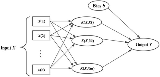
SVM is the way of mapping the sample space into a high-dimensional or infinite dimensional feature space, by using a nonlinear mapping technique. Then the nonlinear separable problem in the original sample is converted into a linear separable problem in feature space. The nonlinear problems that cannot be solved in low dimensional sample space can thus be linearized in high dimensional feature space. In general, increasing the dimension always leads to a more complicated calculation, but SVM solves this problem ingeniously by using the kernel function expansion theorem. Though the problem was established in high dimensional feature space, there is a minimal increase in computing complexity compared to the common linear model. To some extent the “dimension disaster” is actually avoided. The schematic of the SVM is shown in Fig. 3 [26].

Fig. 3The structure of SVM schematic

4.4. Classification algorithm

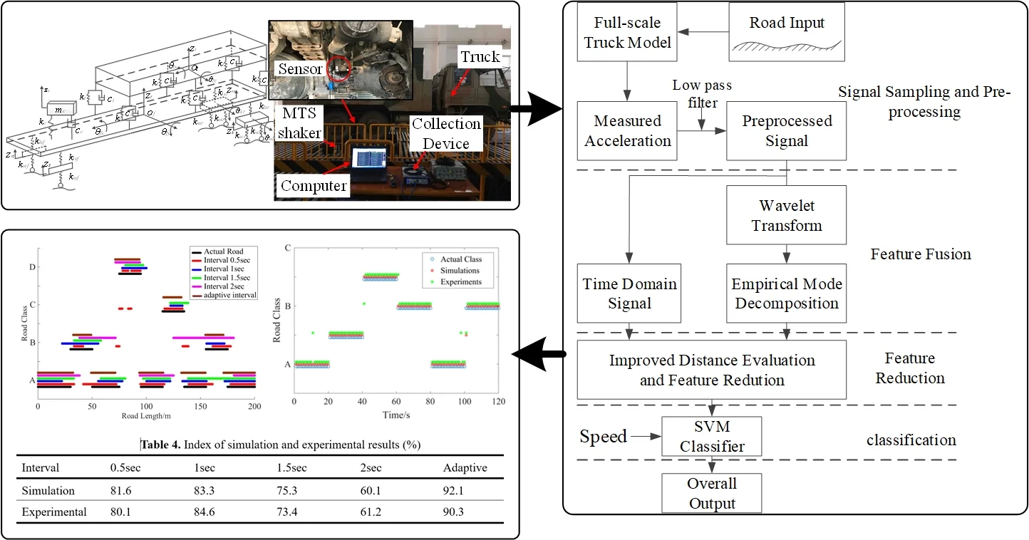
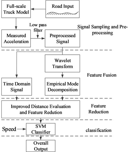
The structure of this process is shown in the Fig. 4, which can be divided into four stages, i.e. signal sampling and pre-processing, feature fusion, feature reduction and classification.

Fig. 4Flow chart of the classification algorithm

5. Simulations

To value the performance of the proposed algorithm, simulations about classification with different speeds and identification intervals are reported in this section. The influence of classification interval was researched and an adaptive interval algorithm for classification was proposed, and simulation results proved that the novel adaptive interval is performance better than fixed interval.

5.1. Classification with different speeds

Under the assumption that the vehicle is traveling along the road with 4 standard levels of velocity (20 km/h, 40 km/h, 60 km/h, 80 km/h) and 8 standard levels of road profiles (ISO level A, ISO level B, ISO level C, ISO level D, ISO level E, ISO level F, ISO level G, ISO level H), there are total 32 kinds of road excitation obtained. 32 kinds of 10 seconds long road excitation condition are generated by using road model method in Section 1.2, then 32 kinds of 10 seconds long truck system responses are obtained. These known road class responses are applied to perform the superior features selection and train the SVM classifier.

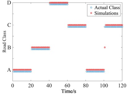
To validate the proposed method, a new 120 seconds road excitation was generated, which is composed of 6 conditions: A class road with 80 km/h vehicle speed; B class road with 60 km/h vehicle speed; D class road with 20 km/h vehicle speed; C class road with 40 km/h vehicle speed; A class road with 20 km/h vehicle speed; and a C class road with 60 km/h vehicle speed. Each condition remains unchanged for 20 seconds and assumes that the translation time of two conditions is neglected. Fig. 5 shows the classification result.

It is seen in Fig. 5 that there was only one error in the 120 identification cycles. The result implies that the classification accuracy of this new-generated road is more than 99 %. It can also be seen that even though vehicles are driven on A class road in time frame 0-20 sec and 80-100 sec with speed 80 km/h and 20 km/h respectively, the classifier can identify that the road class is same (A). Similarly, in the time frames 60-80 sec and 100-120 sec when the vehicle is driven on a C class road with speed 40 km/h and 60 km/h respectively, the classifier also can identify the road class avoiding the speed influence.

Fig. 5Classification results for generated profile

5.2. Influence of identification interval

Considering that under a constant vehicle speed, a shorter identification time interval comes with a shorter road class identification spatial interval. A more accurate road surface analysis is achieved and so, the classifier needs a short identification time interval. However, it is hard to obtain sufficient information for the low frequency components of a signal to classify the road when interval is too short. This is particularly true when the vehicle is driven at low speeds where a short interval may lead to serious identification error.

To discuss the influence of interval size in spatial, a 200 meters road was generated. This is composed of A, B and C class road levels in 9 frames: 30 meters A class road; 20 meters B class road; 25 meters A class road; 20 meters D class road; 20 meters A class road; 20 meters C class road; and 20 meters A class road; and 20 meters B class road; and 25 meters A class road, in successive order. It is assumed that the vehicles drive on the road surface at 20 km/h, 40 km/h, 60 km/h and 80 km/h respectively and the identification intervals are 0.5 sec, 1 sec, 1.5 sec and 2 sec. The actual road surface and the classification of the roads results, for different intervals, are shown in Fig. 6. The varying length lines in Fig. 6 represent the length of one road class in reality or classified. When the vehicle speed is 80 km/h, the classification results for shorter spatial intervals show more accuracy than the result in a longer interval. This is because vehicles travel more than 40 meters in 2 sec, thus it is too long to determine the information of the road-class changes covered. When the interval is 0.5 sec, the vehicle identified the road class about per 11 meters, resulting in a relative high spatial accuracy. When vehicle speed is 20 km/h, the spatial classification results of a 0.5 sec interval was the worst. This is due to the fact that a vehicle only travels circa 5 meters in a 0.5 sec interval, which is too short for the classifier to obtain enough effective road information to make an accurate classification.

In order to evaluate the performances of different classification intervals, a quantitative index is utilized to assess the road surface classification accuracy. This index is:

13

P = \frac{L_{e}}{L} \times 100 %,

where $L_{e}$ is the portion of the classified road (in meters) which is the same as the real road class and $L$ is the total generated road length ( $L =$ 200 m). The index values for different interval durations and vehicle speeds are shown in Table 2. It can be seen that when the vehicle speed is 80 km/h, the spatial accuracy of the road surface identification is reduced with an increase in the time interval. The converse is true when the vehicle speed is 20 km/h. When the speed is 60 km/h, the best interval is 1 second, and when the speed is 40 km/h the best interval is 1.5 second. If considering a more realistic variable vehicle speed, an adaptive length identification interval can be adopted to improve road surface analysis accuracy. That is, a shorter interval for high vehicle speeds and a longer interval for low vehicle speeds.

Fig. 6Classification results of different intervals in for the generated road surface: a) vehicle speed is 20 km/h, b) vehicle speed is 40 km/h, c) vehicle speed is 60 km/h, d) vehicle speed is 80 km/h

Classification results of different intervals in for the generated road surface: a) vehicle speed is 20 km/h, b) vehicle speed is 40 km/h, c) vehicle speed is 60 km/h, d) vehicle speed is 80 km/h

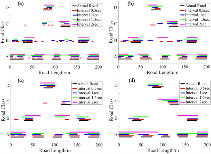
Table 2Index of different classification interval (%)

Interval	0.5 sec	1 sec	1.5 sec	2 sec
20 km/h	73.1	75.4	78.5	87.6
40 km/h	75.4	79.9	84.9	73.6
60 km/h	78.5	84.1	75.1	57.8
80 km/h	87.4	81.6	64.9	55.8

5.3. Adaptive interval

On the basis of Table 2, a large interval was need for enough information for classification accuracy when vehicle run in low speed, but a small interval is enough to maintain information of classification and improve the accuracy in spatial when vehicle run in high speed. Actually, the driver always changes vehicle speed based on different road during the course of ride. Driver may increase the speed when the road is good, and driver often maintain vehicle in low speed when the road is bad. Generally, the fixed classification interval is a compromise of enough information for accurate classification and accuracy in spatial. Thus, an adaptive interval should be employed for obtaining enough information for accurate classification and enough identification accuracy in spatial for road maintenance department. The adaptive interval is that a relatively long interval was used if vehicle run in low speed, and a relatively short interval was used if vehicle speed is high.

Assumption:

1. Assume that vehicle speed is 80 km/h on A level road, vehicle speed is 60 km/h on B level road, vehicle speed is 40 km/h on C level road and vehicle speed is 20 km/h on D level road.

2. The translation time of two different road levels and two speed levels are neglected.

The Fig. 7 shows the simulation results of a vehicle run on the generated 200 meters road in different speed, and the interval is 0.5 second, 1 second, 1.5 second, 2 second and adaptive interval. It can be seen that the brown lines (with adaptive interval) are very proximate with the black lines (actual road). To value the specific performance of different interval, index proposed in Section 4.2 was used, and the index results are shown in Table 3. It can be seen that the adaptive interval is great improving classification accuracy in spatial.

Fig. 7Classification results of different fixed intervals and adaptive interval

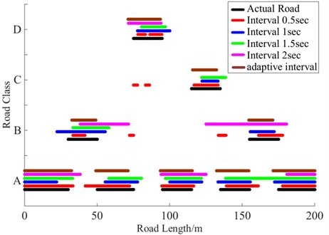
Table 3Index of different fixed intervals and adaptive interval (%)

Interval	0.5 sec	1 sec	1.5 sec	2 sec	Adaptive
Index	81.6	83.3	75.3	60.1	92.1

6. Experimental tests

An experimental system was also developed to verify the proposed method, as depicted in Fig. 8. The system includes: a 13 degree-of-freedom truck with accelerate velocity sensor on; a MTS hydraulic shaker controlled by a PC to provide the road excitation; a collection device for collecting acceleration signals; and a computer for processing the collected signals and classifying the road. The 32 kinds of 10 seconds long road excitation condition was imported into the MTS shaker control system, and the truck system responses were obtained. Then these responses, with known road classes, were applied to perform the superior features selection and train the SVM classifier. In this process, low-frequency parts of the features was not enough to train an accurate classifier, so 100 times truck responses of every kind road conditions were conducted.

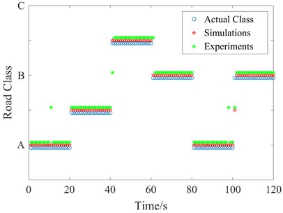
The performance of the proposed method of classifying the road was examined by using the truck responses in experimental. The generated road in Section 4.1 were imported in the MTS shaker control system, and the truck system responses were collected. The tuck system responses are shown in Fig. 9. It can be seen that the first part is close to the second part and the third part is close to the last part, but they are not the same road condition responses. Then we used the proposed classifier to estimate the road levels, and the classification results were contrasted with the real road conditions and simulation results in Fig. 10. It can be seen clearly that the method is very effective, though the results were not accuracy as simulation. The classification accuracy of experimental is as high as 96.7 % (116/120). It can also be seen that even though vehicles are driven on A class road in time frame 0-20 sec and 80-100 sec with speed 80 km/h and 20 km/h respectively, the classifier can identify the road class accurately. Similarly, in the time frames 60-80 sec and 100-120 sec when the vehicle is driven on a C class road with speed 40 km/h and 60 km/h respectively, the classifier also can identify the road class effective. These results indicate that the classifier of this method is superior to others in ability of avoiding the influence of vehicle speed.

Fig. 8Schematic diagram of experimental setup

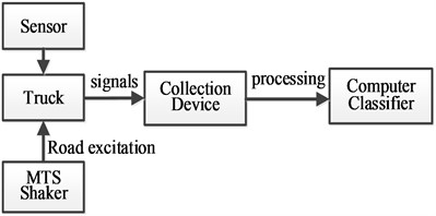
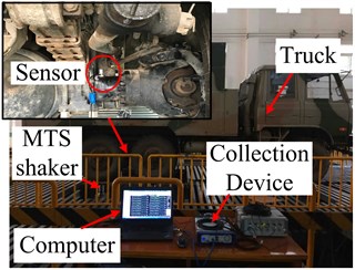
Fig. 9Truck system responses

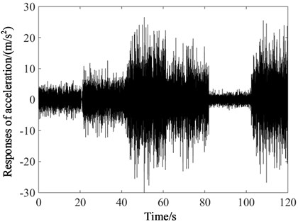
Fig. 10Experimental classification results

Providing the generated road in Section 4.3 to the hydraulic shaker, then the performance of the fixed and adaptive interval of classification was examined. Table 4 show the accuracy index of simulation and experimental, and the experimental results approximate with the simulations results. It can be seen clearly that if the vehicle is driving in the generated road with adaptive speed depending on road class condition, the smaller identify interval can obtain the higher accuracy results in spatial, as the classification accuracy in spatial is influenced by the vehicle speed. The classification accuracy in spatial with the proposed adaptive interval greatly enhanced the ability of avoiding vehicle speed effect. The simulation results and the experimental results proved that the method is effective.

Table 4Index of simulation and experimental results (%)

Interval	0.5 sec	1 sec	1.5 sec	2 sec	Adaptive
Simulation	81.6	83.3	75.3	60.1	92.1
Experimental	80.1	84.6	73.4	61.2	90.3

7. Conclusions

In this paper, an effective method of estimating the road surface condition was presented and an adaptive identification interval was proposed for improving the accuracy in spatial. A new signal processing technique, integrating the Wavelet Transform and Empirical Mode Decomposition, is developed and considers vehicle speed as a parameter of paramount importance in the process. Computer simulations of a full-scale truck model have been carried out to analyses the influence of the classification interval. A special index was proposed to evaluate the algorithm classification accuracy in spatial, and a synthesized 200 m special road classification shows that using a short duration interval in high vehicle speeds and long duration interval in low vehicle speeds is a good way to improve the spatial road classification accuracy. Then an adaptive classification interval was proposed for improving the classification accuracy. Both the simulation results and experimental results verified that the proposed algorithm for estimating the road condition is effective and the classification accuracy in spatial is greatly improved by using adaptive interval.

References

Zhang Z., Deng F., Huang Y., Bridgelall R. Road roughness evaluation using in-pavement strain sensors. Smart Materials and Structures, Vol. 24, 2015, p. 115029.

Publisher
Qin Y., Langari R., Gu L. The use of vehicle dynamic response to estimate road profile input in time domain. ASME Dynamic System Control Conference, 2014.

Search CrossRef
Doumiati M., Victorino A., Charara A., Lechner D. Estimation of road profile for vehicle dynamics motion: experimental validation. Proceedings of the American Control Conference, 2011.

Search CrossRef
Imine H., Fridman L. Road profile estimation in heavy vehicle dynamics simulation. International Journal of Vehicle Design, Vol. 47, 2013, p. 234-49.

Search CrossRef
Mccann R., Nguyen S. System identification for a model-based observer of a road roughness profiler. IEEE Region 5 Technical Conference, 2007.

Search CrossRef
Nordberg T. P. An iterative approach to road profile identification utilizing wavelet parameterization. Vehicle System Dynamics, Vol. 42, 2004, p. 413-32.

Search CrossRef
Gonzalez A., O'brien E. J., Cashell K. The use of vehicle acceleration measurements to estimate road roughness. Vehicle System Dynamics, Vol. 46, 2008, p. 483-99.

Publisher
Qin Y. C., Guan J. F., Gu L. The research of road profile estimation based on acceleration measurement. Applied Mechanics and Materials, Vol. 226, Issue 228, 2012, p. 1614-1617.

Search CrossRef
Koch G., Kloiber T., Lohmann B. Nonlinear and filter based estimation for vehicle suspension control. 49th IEEE Conference on Decision and Control (CDC), 2011.

Search CrossRef
Rabhi A., M'sirdi N. K., Fridman L., Delanne Y. Second order sliding mode observer for estimation of road profile. International Workshop on Variable Structure Systems, 2006.

Search CrossRef
Qin Y., Dong M., Zhao F. Road profile classification for vehicle semi-active suspension system based on adaptive neuro-fuzzy inference system. 54th Annual Conference on Decision and Control, 2015.

Search CrossRef
Tao X., Pengsong W., Yu D. Effect of long-wavelength track irregularities on vehicle dynamic responses. Shock and Vibration, Vol. 2019, 2019, p. 4178065.

Search CrossRef
Zhao F., Ge S. S., Tu F., Qin Y., Dong M. Adaptive neural network control for active suspension system with actuator saturation. IET Control Theory and Applications, Vol. 10, 2016, p. 1696-705.

Publisher
Qin Y., Rath J. J., Hu C., Sentouh C., Wang R. Adaptive nonlinear active suspension control based on a robust road-classifier with a modified super-twisting algorithm. Nonlinear Dynamics, Vol. 97, 2019, p. 2425-2442.

Publisher
Qin Y., Dong M., Feng Z., Liang G. Suspension semi-active control of vehicles based on road profile classification. Dongbei Daxue Xuebao/journal of Northeastern University, Vol. 37, 2016, p. 1138-43.

Search CrossRef
Hammond D. K., Vandergheynst P., Gribonval R. The Spectral Graph Wavelet Transform: Fundamental Theory and Fast Computation. Vertex-Frequency, Analysis of Graph Signals, Springer International Publishing, 2019, p. 141-175.

Publisher
Peng Z. K., Tse P. W., Chu F. L. A comparison study of improved Hilbert-Huang transform and wavelet transform: application to fault diagnosis for rolling bearing. Mechanical Systems and Signal Processing, Vol. 19, 2005, p. 974-88.

Publisher
Attoh-Okine Hilbert-Huang Transform, Profile, Signal, and Image Analysis. John Wiley and Sons, 2017.

Search CrossRef
Mechanical Vibration-Road Surface Profiles -Reporting of Measured Data. 8608 I., International Organization for Standardization, 1995.

Search CrossRef
Dodds C. J., Robson J. D. The description of road surface roughness. Journal of Sound and Vibration, Vol. 31, Issue 2, 1973, p. 175-183.

Publisher
Vantsevich V. V. Road and off-road vehicle system dynamics. Understanding the future from the past. Vehicle System Dynamics, Vol. 53, 2015, p. 137-53.

Publisher
Mastinu G., Ploechl M. Road and off-Road Vehicle System Dynamics Hand Book. CRC Press, 2014.

Publisher
Qin Y. C. Research on Vehicle Semi-Active Suspension System Based on Road Estimation. Beijing Institute of Technology, Beijing, 2016.

Search CrossRef
Wang L. M., Shao Y. M. Crack fault classification for planetary gearbox based on feature selection technique and K-means clustering method. Chinese Journal of Mechanical Engineering, Vol. 31, 2018, p. 242-52.

Publisher
Cortes C., Vapnik V. Support-vector networks. Machine Learning, Vol. 20, 1995, p. 273-97.

Publisher
Wang Xc, Shi F., Yu L. Matlab Neural Network 43 Case Analysis. Beihang University Press, Beihang, 2016.

Search CrossRef

Cited by

A road level identification method for all-terrain crane based on Support Vector Machine

Guoqiang Wang | Wentao Qu | Chunsi Chen | Zeren Chen | Yi Fang

(2022)

About this article

Received

11 December 2019

Accepted

24 March 2020

Published

30 September 2020

SUBJECTS

Vibration in transportation engineering

DOI

https://doi.org/10.21595/jve.2020.21222

Keywords

road excitation classification

wavelet transform

empirical mode decomposition

system response

spatial accuracy

This is an open access article distributed under the Creative Commons Attribution License, which permits unrestricted use, distribution, and reproduction in any medium, provided the original work is properly cited.

Previous article in issue Previous Next article in issue Next

Research article

2024 01 21

Rolling bearing fault diagnosis based on variational mode decomposition and weighted multidimensional feature entropy fusion

Na Lei, Feihu Huang, Chunhui Li

Research article

2018 09 24

Vibration signal de-noising based on empirical wavelet transform autocorrelation analysis

Jiajia Han, Jide Jia, Xiangyu Jia, Gang Ren

Research article

2018 06 30

Gear fault feature extraction and classification of singular value decomposition based on Hilbert empirical wavelet transform

Rahmoune Chemseddine, Merainani Boualem, Benazzouz Djamel, Fedala Semchedine

Research article

2017 12 31

Fault diagnosis of rotor using EMD thresholding-based de-noising combined with probabilistic neural network

Dong Liu, Hongtao Zeng, Zhihuai Xiao, Lihong Peng, O. P. Malik

X. Dang, L. Zhou, X. Wei, and Y. Wang, “A road quality classification technique based on vehicle system responses with experimental validation,” Journal of Vibroengineering, Vol. 22, No. 6, pp. 1481–1494, Sep. 2020, https://doi.org/10.21595/jve.2020.21222

Copy Extrica

Copied to clipboard!

TY  - JOUR
DO  - 10.21595/jve.2020.21222
UR  - https://doi.org/10.21595/jve.2020.21222
TI  - A road quality classification technique based on vehicle system responses with experimental validation
T2  - Journal of Vibroengineering
AU  - Wang, Yushuai
AU  - Dang, Xiaozheng
AU  - Zhou, Liangsheng
AU  - Wei, Xiaojun
PY  - 2020
DA  - 2020/09/30
PB  - JVE International Ltd.
SP  - 1481-1494
IS  - 6
VL  - 22
SN  - 1392-8716
SN  - 2538-8460
ER  - 

Copy Ris

Copied to clipboard!

@article{Wang_2020,
	doi = {10.21595/jve.2020.21222},
	url = {https://doi.org/10.21595/jve.2020.21222},
	year = 2020,
	month = {sep},
	publisher = {{JVE} International Ltd.},
	volume = {22},
	number = {6},
	pages = {1481--1494},
	author = {Yushuai Wang and Xiaozheng Dang and Liangsheng Zhou and Xiaojun Wei},
	title = {A road quality classification technique based on vehicle system responses with experimental validation},
	journal = {Journal of Vibroengineering}
}

Copy Bibtex

Copied to clipboard!

[1]Y. Wang, X. Dang, L. Zhou, and X. Wei, “A road quality classification technique based on vehicle system responses with experimental validation,” Journal of Vibroengineering, vol. 22, no. 6, pp. 1481–1494, Sep. 2020, doi: 10.21595/jve.2020.21222.

Copy IEEE

Copied to clipboard!

Wang, Yushuai, Xiaozheng Dang, Liangsheng Zhou, and Xiaojun Wei. “A Road Quality Classification Technique Based on Vehicle System Responses with Experimental Validation.” Journal of Vibroengineering 22, no. 6 (September 30, 2020): 1481–94. https://doi.org/10.21595/jve.2020.21222.

Copy Chicago

Copied to clipboard!

A road quality classification technique based on vehicle system responses with experimental validation

Abstract

Highlights

1. Introduction

2. System models

2.1. Vehicle model

2.2. Road model

2.2.1. Road irregularities

2.2.2. Road characteristics in the transverse direction

2.2.3. Road high profile modeling

2.2.4. Two-track excitations

3. Feature definition

4. Classification algorithm

4.1. Signal sampling and pre-processing

4.2. Feature reduction

4.3. Classifier (SVM)

4.4. Classification algorithm

5. Simulations

5.1. Classification with different speeds

5.2. Influence of identification interval

5.3. Adaptive interval

6. Experimental tests

7. Conclusions

References

Cited by

About this article

Related Articles