Abstract
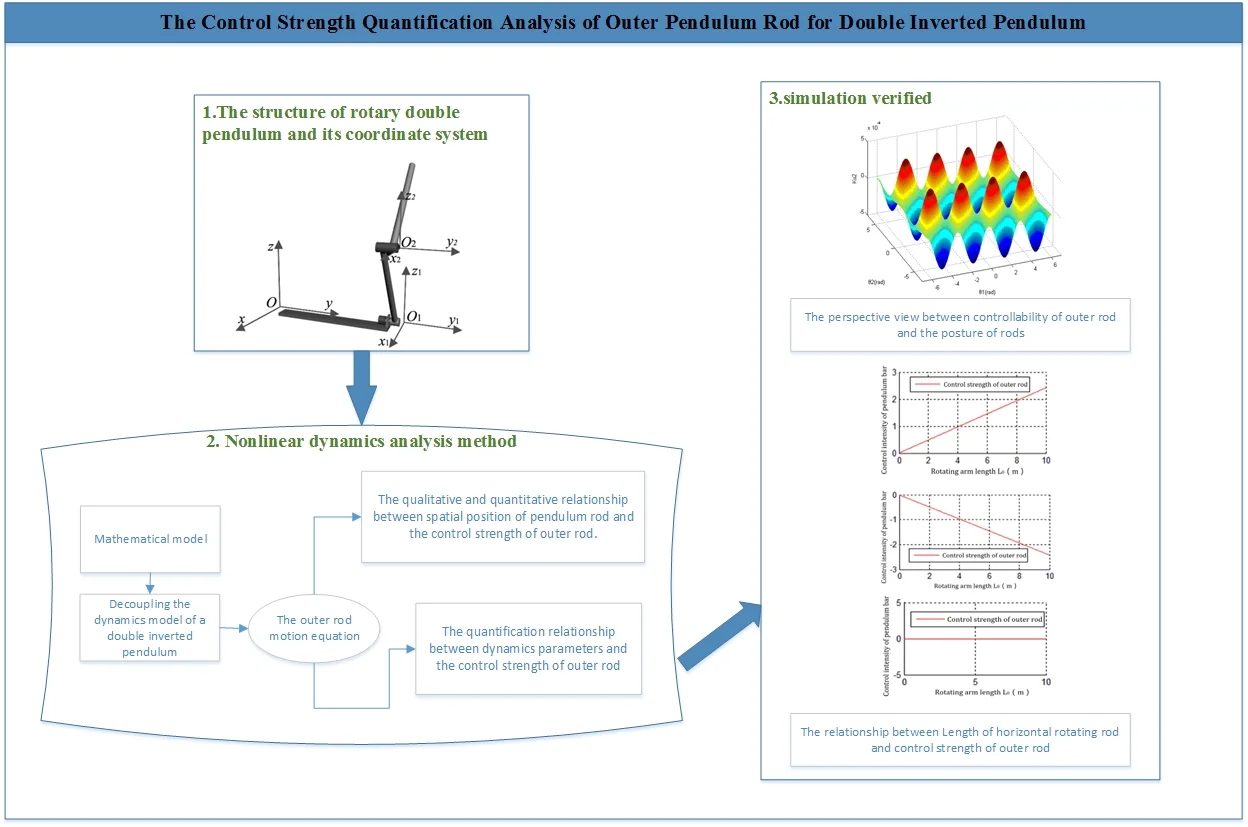
Due to the complexity of the dynamics characteristics of an inverted pendulum, and the problem that the linearization analyze method cannot satisfy the controlling requirement, a nonlinear dynamics analyze method was proposed. Through decoupling the dynamics model of a double inverted pendulum, the outer pendulum rod motion equation was derived. And then, aiming at the control strength function of outer pendulum rod, the qualitative and quantitative relationship between spatial position of pendulum rod and the control strength of outer rod, and the quantification relationship between dynamics parameters and the control strength of outer rod were separately analyzed. And the simulation verified the correctness of the analysis.
Highlights
- The structure of rotary double pendulum and its coordinate system
- Nonlinear dynamics analysis method
- simulation verified
1. Introduction
The inverted pendulum is a classical underactuated mechanical system with nonholonomic constraints. Such kind of non-completely controllable system is important for the dynamics characteristic analysis. In article [1], the method based on Lyapunov stability theorem to conduct the stability control of rotating inverted pendulum was adopted. Jiang built up the mathematical model for rotary inverted pendulum with Lagrange function [2]. The parameter identification for the physical model of two-link and three-link was done through the least square method [3, 4]. The stability control of triple inverted pendulum with cloud control method was realized in [5]. And the stability control of quadruple inverted pendulum with variable universe fuzzy control algorithm was firstly realized in [6]. The controllability of double inverted pendulum and triple inverted pendulum close to equilibrium points with linearization method was analyzed in [4, 8]. But it is not suitable for the area except equilibrium point. Liu applied the Lyapunov exponent formed by state equation to express the motion stability of the system [9]. It is an efficient method to evaluate the quality of closed-loop system after the fact. But with little valueness for designing the controlling system beforehand. The angular acceleration expression of passive joint was derived through dynamics decoupling for a class of rootless underactuated systems in [10]. And simulation and analysis of the controllability of passive joint were carried out. But the quantification relationship between control input and passive joint did not get further discuss. Also, the quantification relationship between physical parameters and system controlling characteristics did not get further study in most relative researches.
The article mainly discussed the control strength quantification analysis of outer pendulum rod for double inverted pendulum. In Section 2, through decoupling the dynamics model, the outer pendulum rod action strength function was derived. In Section 3, the strength analysis, including maximum positive control and maximum negative control, of the outer pendulum rod and the quantification analysis of dynamics parameters and control strength of the outer rod were mainly discussed. Section 4 includes the discussion and analysis of simulation results. Section 5 presents the concluding remarks.
2. Mathematical model and dynamics decoupling
2.1. Mathematical model
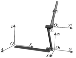
The coordinate system was established shown in Fig. 1.
From [11], the mathematical model of the double inverted pendulum can be derived as:
where:
The state variables and physical parameters of the rotating secondary inverted pendulum were defined as follows: , , are the mass of inner rod, outer rod and encoder. , are the centroid position of inner and outer rod. , are the length of horizontal rotating rod and inner rod. , are the rotational friction of cart-inner rod and inner rod-outer rod axis. , represent the moment of inertia of inner and outer rod. , , represent the angle of the horizontal rotating rod, and the inner and outer rod. , , represent the angular speed of the horizontal rotating rod, and the inner and outer rod. And is the control variable.
Fig. 1The structure of rotary double pendulum and its coordinate system
2.2. Dynamics decoupling
The meaning of the physical parameters abbreviation in the mathematical model, and the derivation of the outer rod motion equation are shown as follows:
Then, the expressions of the intensity function factor in Eq. (2) is shown as follow:
3. Quantitative analysis of spatial position of rod and control strength of the outer rod
is a continuous derivable function. Therefore:
Substituting Eq. (4) into :
3.1. Analysis of maximum positive control strength for outer rod
In Eq. (7), the is the relative maximum, when the outer rod angle is .
Considering that is a continuous derivable function, the derivative is zero at the relative maximum value of . Then, can be obtained in Eq. (8).
Substitute into Eq. (7): .
For any given , if the inner rod angle , achieves the highest controllability.
Substitute into Eq. (8): , and:
When , Eq. (10) is the global maximum. Then, , and . The spatial position of inner and outer rods are shown in Fig. 2.
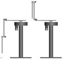
For the same reason, Eq. (9) is the global maximum when . At this time, the outer rod angle and the inner rod angle shown in Fig. 3.
Fig. 2The angle of both rods on max Ku2 when 2k2k3-k1k4>0
Fig. 3The angle of both rods on max Ku2 when 2k2k3-k1k4<0
3.2. Analysis of maximum negative control strength for outer rod
For the same reason, the minimum value can be obtained in Eq. (11):
In Eq. (12), for any given , the outer rod obtains the reverse maximum controllability when . In Eq. (13), , shown in Fig. 4. In Eq. (14), , the inner rod angle shown in Fig. 5.
Fig. 4The angle of both rods on min Ku2 when 2k2k3-k1k4>0
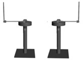
Fig. 5The angle of both rods on min Ku2 when 2k2k3-k1k4<0
3.3. Quantification analysis of dynamics parameters and control strength of outer rod
It can be inferred from the Eq. (15) that has no relationship with the control strength of outer rod . Besides that, simulations of dynamics parameters including rotating arm length , the inner rod mass , the outer rod length and mass , are shown in Section 4.
The relationship of inner rod mass and control strength of outer rod can be simplified as:
It is clear that . When , , , the decrease with . When , , , increases with , if , decreases before passing zero point. When , , , decreases with . When , , increases with , if , decreases before passing zero point.
Also, the relationship between and can be simplified as:
The analyzing process is similar to . With different dynamics parameters, three situations such as increasing, decreasing, decreasing first and then increasing exist for the control strength of outer rod. The simulation under different spatial position is given in Section 4.
4. The simulation verification of control strength for outer rod
In order to verify the analysis process and conclusion mentioned above, the equivalent dynamics parameters [11] were put into Eq. (3). Then, calculate the within the range of pendulum angles . Finally, the 3D surface graphs were drawn as follow.
Fig. 6 and Fig. 7 show the relationship between and rod angles from different perspectives. In these figures, the red area indicates the part in which is greater (the deep red shows the maximum of ). And the blue area is the part which is smaller. Also, when reaches the maximum, the outer rod angles could be , and the inner rod angles could be , . And when reaches the minimum, the outer rod angles could be , and the inner rod angles could be , . Finally, the rod angles with the maximum and the minimum of from Fig. 7 fit the rod angles derived from Eq. (10) and Eq. (13) separately which verified the correctness of analysis about the extremum of mentioned above.
The simulation result of control strength of outer rod and dynamics parameters including , , , and , were separately shown in Fig. 8, Fig. 9, Fig. 10 and Fig. 11.
Fig. 6The perspective view between Ku2 and θ1, θ2
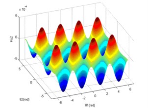
Fig. 7The left and right view between Ku2 and θ1, θ2
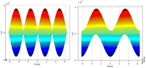
Fig. 8The relationship between L0 and Ku2
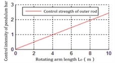
a) Inverted point
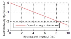
b) Hanging point
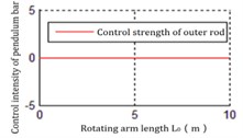
c) Horizontal point
Fig. 9The relationship between l2 and Ku2
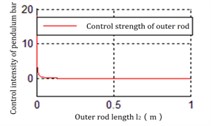
a) Inverted point
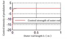
b) Hanging point
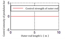
c) Horizontal point
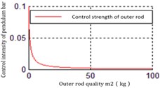
Fig. 10The relationship between the mass of inner rod m1 and Ku2
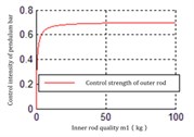
a) Down point, increases with
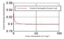
b) Spatial position of rods (80°, 110°), decreases with
It can be inferred from those figures that the dynamics parameters are positively or negatively correlated with . For the parameters , , the influence for is much greater than , . And the hardly changes with , . Hence, adjusting could be the main method to satisfy . However, in the actual system, the improvement of the control action intensity does not mean that the control difficulty is low. And it is also necessary to comprehensively consider that the dynamic and static characteristics such as the servo precision and response speed of the drive mechanism (motor, controller, transmission mechanism).
Fig. 11The relationship between the mass of inner rod m2 and Ku2
a) Down point, decreases with
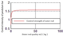
b) Spatial position of bars (80°,110°), increases with
5. Conclusions
In this article, the control strength quantification analysis of the outer pendulum rod for double inverted pendulum was mainly discussed from two perspectives. One is the qualitative and quantitative relationship between the control strength of the outer rod and the spatial position of the pendulum rod. And the other is the quantification relationship between the control strength of the outer rod and the dynamics parameters (including the length of pendulum rod , , , and the mass of pendulum rod , ). Finally, the correctness of the relationship was illustrated by simulation results.
References
-
Wen Jie, Shi Yuanhao, Lu Xiaonong Stabilizing a rotary inverted pendulum based on logarithmic Lyapunov function. Journal of Control Science and Engineering, Vol. 2017, 2017, p. 4091302.
-
Jiang Xiangju, Liu Erlin Research and realization of the initial and stable pendulum of rotating inverted pendulum. Journal of Process Automation Instrumentation, Vol. 9, 2016, p. 6-9.
-
Zhu Qiuguo, Wu Haoxian, Yi Jiang, Xiong Rong, Wu Jun Push recovery for humanoid robots with passive damped ankles. Proceedings of the IEEE Conference on Robotics and Biomimetics, Zhuhai, China, 2015, p. 1578-1583.
-
Zhu Qiuguo, Wu Haoxian, Wu Jun, Xiong Rong Humanoid robot standing balance control based on three-link dynamics model. Journal of Robot, Vol. 4, 2016, p. 451-457.
-
Zhang Feizhou, Li Yide Realization of intelligent control of inverted pendulum with cloud model. Journal of Control Theory and Applications, Vol. 4, 2000, p. 519-523.
-
Miao Zhihong, Li Hongxing Fuzzy control of robust guaranteed cost of plane motion N-th inverted pendulum. Journal of Huazhong University of Science and Technology (Natural Science Edition), Vol. 3, 2014, p. 62-74.
-
Bo Guizhen, Mei Xiaorong, Wang Shuyi Establishment of mathematical model and controllability of triple inverted pendulum on inclined orbit. Journal of Electric Machines and Control, Vol. 2, 2003, p. 170-173.
-
Dan Yuanhong, Lai Hongxia Modeling and analysis of observability and controllability of annular double inverted pendulum. Journal of Chongqing University of Technology (Natural Science), Vol. 11, 2007, p. 7-16.
-
Liu Yunping, Li Yu, Chen Cheng, Zhang Yonghong Stability of nonholonomic system based on lyapunov index. Journal of Huazhong University of Science and Technology (Natural Science Edition), Vol. 12, 2016, p. 98-101.
-
Li Na, Zhao Tieshi, Jiang Haiyong, Wang Jiazhong Dynamics coupling characteristics of rootless underactuated redundant robots. Journal of Mechanical Engineering, Vol. 9, 2016, p. 49-55.
-
Dan Yuanhong, Xu Peng, Zhang Wei, Tan Zhi Improved genetic algorithm for parameters identification of cart-double pendulum. Journal of Vibroengineering, Vol. 21, Issue 6, 2019, p. 1587-1599.
About this article

