Abstract
In this paper, the method based on Laplace transform and Fourier transform and their inverse transforms is developed to give an exact solution to the forced torsional vibration of a shaft subjected to multiple inertias, multiple elastic supports, arbitrary boundary conditions and arbitrary excitation forces. Two simple cases are used to show in detail how this developed method can obtain an exact analytical solution to the forced torsional vibration of shaft and the results are compared with Eigenfunction Expansion Method and Finite Element Method (FEM) to demonstrate the accuracy and effectiveness of the developed method. Two more complex cases are investigated to further show the superiority of the developed method over FEM in highly efficient and accurate. Finally, using the developed method, the effects of parameters on forced torsional vibration response of shaft are discussed, including the stiffness, the location of elastic supports and the time interval of impact loading. The developed method can provide a reliable theoretical base not only for analysis and fault diagnosis of a shaft system in engineering signal testing projects but also for the verification of other numerical and analytical methods.
Highlights
- The forced torsional vibration of a shaft subjected to multiple inertia, multiple elastic supports, arbitrary boundary conditions and arbitrary excitation forces is studied
- A new method is developed to give an exact solution based on Laplace transform and Fourier transform and their inverse transforms
- The accuracy and effectiveness of the developed method have been demonstrated
- The effects of parameters on forced torsional vibration response of shaft are discussed, including the stiffness, the location of elastic supports and the time interval of impact loading
1. Introduction
A shafting system is an important component in the structures widely used in aviation, navigation, machinery, etc. The torsional vibration is a common cause of the failure of the shaft system. Hence, studying the characteristics of the torsional vibration of a shaft is important. It can not only provide the ideas for the engineering design of the shaft system but also the basis for fault diagnosis. Usually, the study is to deal with a forced torsional vibration of a simplified shaft system with multiple concentrated inertias and multiple elastic supports.
There is a lot of published literature available involving in the forced torsional vibration of the shaft system. Among them, the energy method and the amplification factor method were the most basic and important methods widely used to study torsional vibration [1]. The Holzer method was often used for forced torsional vibration as well [2, 3]. With the rapid development of computer technology, the system matrix method, the transfer matrix method and FEM have been widely used in [4, 5]. Meanwhile, many approximate solutions have also been developed by researchers. Based on the a modified Riccati torsional transfer matrix combining with the Newmark- method, Xiang et al. [6] presented an analytical method of the forced torsional vibrations of a Shafting System under Electrical Disturbances. The torsional vibration of an elastic rod with external dry friction was solved using approximate methods of expansion in a small parameter and harmonic linearization by Koibin [7]. A general analytical solution was developed to study vibration of non-uniform Timoshenko beams coupled with flexible attachment and multiple discontinuities based on separation of variables in conjunction with the transfer matrix approach by Zhang et al. [8]. Ewing and Mirsafian [9] proposed an analytical model consisting of two Euler-Bernoulli beams joined by a torsional spring with linear and cubic stiffness and a method of harmonic balance was used to give an approximate solution for the model with pinned-fixed conditions. Jiang et al. [10] discussed the forced tensile and torsional response of helical springs caused using the Laplace transforms. The nonlinear torsional vibration dynamical modeling of the multi-DOF rolling mill’s main drive system is established by Han et al. [11] and the amplitude-frequency characteristic equations are obtained by multiscale method. Beytullah et al. [12] investigated the dynamic behavior of composite cylindrical helical rods subjected to time-dependent loads in the Laplace domain. Bapat and Bhutani [13] have developed a general approach for free and forced vibrations of stepped systems governed by the One-Dimensional wave equation with non-classical boundary conditions. Wang et al. [14] studied forced torsional vibration of a finite class 622 piezoelectric hollow cylinder with free-free ends subjected to dynamic shearing stress and time dependent electric potential at both internal and external surfaces by means of the superposition method and the separation of variables technique. On the basis of lumped parameter model and the Lagrange method, the dynamic analysis and multi-object optimization of the forced torsional vibration for vehicular multi-stage planetary gears was studied by Liu Hui et al. [15]. Kang and Hoon [16] investigated hysterically damped free and forced vibrations of axial and torsional bars using a closed form exact method. Rudavskii et al. [17] studied the forced flexural-and-torsional vibrations of a cantilever beam of constant cross section. Torsional vibrations of composite bars of variable cross-section by BEM are investigated by Sapountzakis [18]. Among the researches, the numerical approach is common used to solve the problems of forced torsional vibration. Hardly, one can found an actual analytical solution. Yang [19] developed an analytical method with a distributed transfer function formulation and a residue formula for inverse Laplace transform for transient vibration analysis of stepped systems composed of shafts and strings carrying lumped masses. In Ref. [19], the matching conditions are given to describe the discontinuity at the locations of lumped mass and elastic supports and to obtain the forced vibration response of the equation the natural frequencies needs to be solved first.
In this paper, a method based on Laplace transform and Fourier transform defined on a bounded interval is developed to obtain an exact solution to the forced torsional vibration of a shaft with multiple concentrated inertias and elastic supports deal with arbitrary boundary conditions and arbitrary excitation forces. Different from Ref. [19], in this study the delta function is used to describe the discontinuity at the locations of lumped mass and elastic supports and the forced vibration response can be obtained directly. First, the developed method is introduced in detail. Then, two examples, a shaft with two different forms of excitation and different boundary conditions, are used to show in detail how this developed method can obtain an exact analytical solution to the forced torsional vibration of the shaft. The results are compared with the widely accepted Eigenfunction Expansion Method and FEM to demonstrate the accuracy and effectiveness of the developed method. Furthermore, to further show its superiority over FEM, a shaft with a single circular disc under the general excitation force and a shaft with one elastic support under the impact loading are studied. To take advantage of the developed method further, the influence of different parameters on the torsional forced vibration response of shaft is discussed. They include the stiffness, the position of elastic supports and the time interval of the impact loading.
2. Developed method
2.1. Free vibration equation of a shaft
The torsional free vibration equation of a shaft with multiple concentrated inertias and elastic supports (with arbitrary magnitudes and locations) subjected to arbitrary boundary conditions can be obtained from the Hamilton’s principle or from the equation of motion. It is given as follows:
where the axis is along the shaft axis. and are the second derivative of with respect to and , respectively. The partial derivative of is . The length and the radius of the circular section of the shaft are and , respectively. The shear modulus is and the mass density is . The polar moment of inertia of the cross section is . The shaft is composed of discs and elastic-supports. is the moment of inertia with the associated -th disc. is the stiffness with associated -th elastic-support. , the torsion angle of each section in the Cartesian coordinate system, is a function of the generalized coordinate and time . It is worth to note that specially, the function is used to characterize the existence of a concentrated inertia and/or an elastic support at certain position. shows -th disc existing at the position and shows -th spring existing at the position . In the following section, a method is developed to solve the equation of forced torsional vibration.
2.2. A developed method to solve forced torsional vibration of shaft
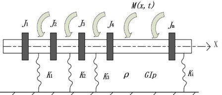
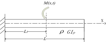
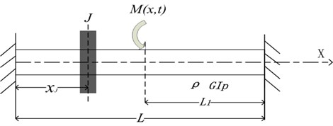
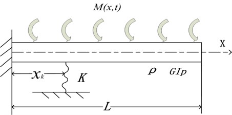
Based on Laplace transform and Fourier transform defined on a bounded interval, a new analytical method is developed herein to solve the forced torsional vibration of a shaft as shown in Fig. 1. The shaft is treated as a beam which can be subjected to multiple concentrated inertias, multiple elastic supports with arbitrary magnitudes and locations and arbitrary boundary conditions and excitations.
Fig. 1A shaft with multiple concentrated inertias and elastic supports under arbitrary excitation
Based on Eq. (1), the motion equation of forced torsional vibration of a shaft is given by the following equation:
where is the applied torque.
The boundary conditions at fixed ends are given as:
The boundary conditions at free ends are given as follows:
The initial angular displacement and the initial angular velocity are given as follows:
Eq. (2) is a second order partial differential equation with the two variables: position and time .
To solve Eq. (2), first step is to separate the variables and . To begin with, the Laplace transform of Eq. (2) with respect to time gives:
where is the Laplace transform parameter:
Substituting the initial conditions of Eq. (7) into Eq. (8) yields:
Since Eq. (11) is a second order non homogeneous equation with constant coefficient and contains Dirac Delta function, it will be very complex to be solved. Therefore, a developed approach to solve this equation is to make Fourier transformation of Eq. (11) with respect to the variable . Considering in the range of [0, ], the Fourier transform defined on this bounded interval can be described by the following relationship:
where is the Fourier transform parameter. The Fourier transform of Eq. (11) with respect to gives:
In which:
If both ends of shaft are fixed, substituting the boundary conditions of Eq. (3) and Eq. (4) into the Eq. (13) leads to:
where .
The inverse Laplace transform of Eq. (17) gives:
where is the inverse of . The symbol “” represents the convolution operation.
To solve Eq. (18), first, substituting the boundary conditions of Eq. (3) and Eq. (4) into Eq. (18), from , and can be obtained. Then similarly, substituting into Eq. (18), the values of and can be obtained. After that, the function of can be obtained. Based on the residue theorem, the exact function of can be derived by inverse Laplace transform of . Hence, the forced torsional vibration of a shaft is solved.
In the following section, two cases are studied in detail to show how to use this developed method to obtain an exact analytical solution and the results will be compared with the Eigenfunction Expansion Method [20] and the FEM to demonstrate the superiority of the developed method in the accuracy and effectiveness. All the calculations are obtained by MATLAB and the results of FEM are obtained by ANSYS. Using ANSYS, the shaft studied is divided into 60 Timoshenko beam elements (BEAM188) and 61 nodes. The disk is simulated using MASS21 and the spring is simulated ideally by linear stiffness element (SPRING14). For the purpose of brief, all these will not be mentioned later on.
3. Method validation
The first case is a shaft fixed at both ends and subjected to the distributed loading. The second case is a shaft with one end clamped and the other free and subjected to a concentrated loading at the center of the shaft.
3.1. Case one
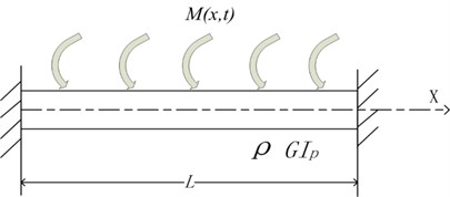
Case 1 is a shaft fixed at both ends and subjected to the distributed uniform moment loading as shown in Fig. 2. The shaft has a circular cross-section with the diameter 0.0375 m and the length 3 m. The material properties of the shaft are given as follows. The shear modulus is 81.5×10⁹ N/m2 and the mass density is 7850 kg/m3. The polar moment of inertia of the cross section is . The distributed loading is N⋅m.
Fig. 2A shaft fixed at both ends under distributed loading
The vibration equation, the boundary condition and the initial condition are:
First, Laplace transformation of Eq. (19) with respect to time gives:
Substituting the initial conditions into Eq. (20) leads to:
Eq. (21) can be transformed in accordance with the Fourier transformation rules on a bounded interval as follows:
Substituting the fixed boundary conditions into Eq. (22) leads to:
The inverse Fourier transform of Eq. (23) yields:
Substituting , into Eq. (24), the boundary conditions of are:
From Eq. (25), one can obtain:
Substituting Eq. (26) into Eq. (24) yields:
Inverse Laplace transform of Eq. (27) yields an exact analytical solution of Case 1:
The result of Case 1 by Eigenfunction Expansion Method is given as:
where:
Table 1Amplitude of the center of the beam in Case 1
Method | Amplitude (m) | Difference (%) |
The developed method | 1.3376e-5 | – |
The eigenfunction expansion method | 1.3372e-5 | 0 |
The finite element method | 1.3331e-5 | 0.3364 |
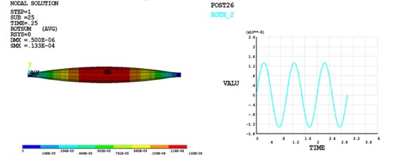
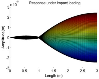
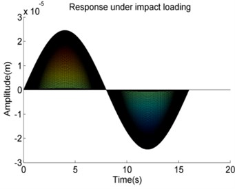
The results from the developed method are shown in Fig. 3(a). The results from the Eigenfunction Expansion Method are shown in Fig. 3(b). Fig. 3(c) shows the results from FEM. In Fig. 3(a), Fig. 3(b) and Fig. 3(c), two figures are the amplitude vs the length of the beam and the amplitude of the center of the beam vs time, respectively. The forced vibration response amplitude of the center from three methods is given in Table 1. It can be seen that the results of the shafting forced vibration response spectrum obtained by the developed method agree well with the Eigenfunction Expansion Method and the FEM.
The developed method shows highly efficient. With simple cases like Case 1 to achieve the desired accuracy, it is just taken one second for the developed method while several minutes for the FEM. As for the Eigenfunction Expansion Method, it needs iterative more than 50 times. The superiority of the developed method over the Eigenfunction Expansion Method and the FEM in accuracy and computation time is obvious.
Fig. 3Results of Case 1
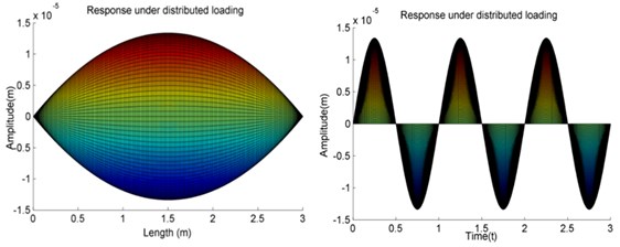
a) The developed method
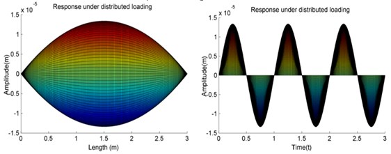
b) The eigenfunction expansion method
c)The finite element method
3.2. Case two
Case 2 shown in Fig. 4 is a shaft with one end clamped and the other free subjected to a concentrate load ae the center. All geometrical and material parameters are same as given in Case 1. The concentrated load is N⋅m.
Fig. 4A shaft with one end clamped and the other free under concentrated loading
The vibration equation, the boundary condition and the initial condition are:
First, Laplace transformation of Eq. (31) with respect to time gives:
Substituting the initial conditions in Eq. (31) into Eq. (32) leads to:
Eq. (33) can be transformed in accordance with the Fourier transformation rules on a bounded interval as follows:
Substituting the boundary conditions in Eq. (31) into Eq. (34) leads to:
Inverse Fourier transform of Eq. (35) yields:
Substituting , into Eq. (36), the boundary conditions of are:
From Eq. (37) one can obtain as follows:
Substituting Eq. (38) into Eq. (36) yields:
Then the exact analytical solution of Case 2 can be obtained by Inverse Laplace transform of Eq. (39):
Table 2Amplitude of the center of the beam in Case 2
Method | Amplitude (m) |
The developed method | 5.9251e-6 |
The finite element method | 5.9247e-6 |
Difference (%) | 0 |
Fig. 5The results of Case 2
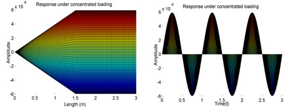
a) The developed method
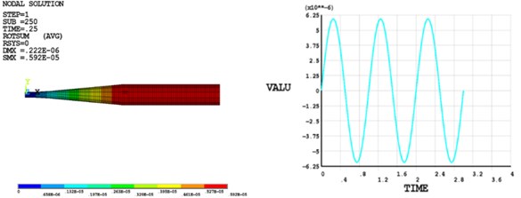
b) The finite element method
The results from the developed method are shown in Fig. 5(a). Fig. 5(b) shows the results from FEM. In Fig. 5(a) and Fig. 5(b), two figures are the amplitude vs the length of the beam and the amplitude of the center of the beam vs time, respectively. The forced vibration response amplitude of the center is given in Table 2. It can be seen that the results obtained by the developed method agree well with the FEM. Case 2 not only again demonstrates the superiority of the developed method in precision and time consuming but also indicates that the developed method is suitable for shafting models with arbitrary boundaries.
4. Complex cases
In this section, the more complicated cases, the torsional forced vibration of a shaft with concentrated inertias and elastic supports, will be investigated to further demonstrate the superiority of the developed method is highly efficient and accurate. First, Case 3, a shaft with single concentrated inertia subjected to random loading, is studied. Then, Case 4, a shaft with an elastic support under impact loading, is studied. The amplitude and the vibration response derived from the developed method are taken to compare with FEM. Finally, to take advantage of the developed method further, the influence of different parameters on forced torsional vibration response of shaft is discussed. The different parameters include the stiffness and position of elastic supports and the time interval of the impact loading.
4.1. Case 3
Case 3, a shaft with single concentrated inertia is fixed at both ends and subjected to a random load, is investigated as shown in Fig. 6. All geometrical and material parameters are same as given in Case 1. The concentrated inertia locates at 1 m. The moment is 0.6021 kg⋅m2. The random loading is N⋅m.
Fig. 6A shaft with a single concentrated inertia fixed at both ends under random loading
The vibration equation, the boundary condition and the initial condition are:
For the sake of brief, omitting the process detail of solving the equation mentioned in Section 2.2, the exact solution of Case 3 is given as follows:
Table 3Amplitude of the center of the beam in Case 3
Method | Amplitude (m) |
The developed method | 2.9625e-6 |
The finite element method | 2.9611e-6 |
Difference (%) | 0 |
Fig. 7The vibration pattern of Case 3 from the developed method
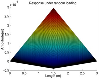
a)
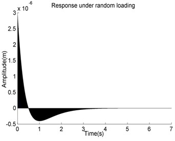
b)
Fig. 8The vibration response spectrum of Case 3 from FEM
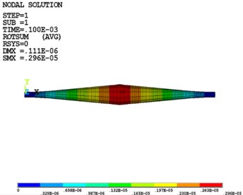
a)
b)
The results of vibration response are shown in Fig. 7. The spectrum diagram of the forced vibration response along the axial direction is given in Fig. 7(a) and the torque of the shaft vs time is given in Fig. 7(b). The torque of is applied at the center of the shaft. The results of the vibration response of FEM are given in Fig. 8. The spectrum diagram of the forced vibration response along the axial direction is given in Fig. 8(a) and the torque of the shaft vs time is given in Fig. 8(b). The vibration amplitude is given in Table 3. All the results from the developed method agree with the FEM very well and once again demonstrate the reliability of the developed method. One can conclude that the developed method is capable and suitable for solving shaft problems in engineering for the arbitrary boundary conditions and excitation.
4.2. Case 4
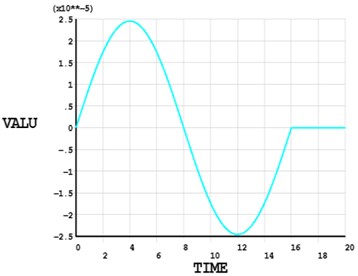
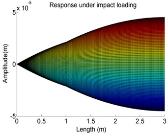
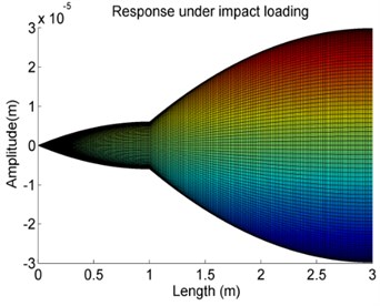
Case 4 is a shaft with an elastic support and one end clamped and the other free subjected to uniform impact loading as shown in Fig. 9. All geometrical and material parameters in this case are the same as given in Case 1. The stiffness of elastic support is 10000000 N/m. The elastic support is located at 1 m. The uniform load is N⋅m, in which represents the starting time of the torque action and is the ending time of the torque action.
Fig. 9A shaft with an elastic support and one end clamped and the other free under impact loading
The vibration equation, the boundary condition and the initial condition are:
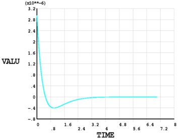
Again, for the sake of brief, omitting the process detail of solving the equation, the exact solution of Case 4 is given as:
where:
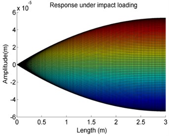
The results are given in Fig. 10(a) and Fig. 10(b). The response amplitude changes along the axial direction as shown in Fig. 10(a). As the big bearing stiffness, the response spectrum of the shaft between 0-1 m is much similar than the rest part of the shaft. The response spectrum of the shaft between 0 to 1 m is similar to that of a shaft with both fixed ends like Case 1 and the response spectrum of the shaft between the 1 m to 3 m is similar to that of a shaft with one end fixed and the other free like Case 2.
Fig. 10The vibration pattern of Case 4 from the developed method
a)
b)
Table 4Amplitude of free end of the beam in Case 4
Method | Amplitude (m) |
The developed method | 2.4513e-6 |
The finite element method | 2.45501e-6 |
Difference (%) | 0.1511 % |
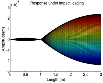
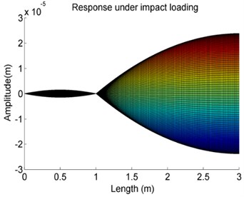
The results from the FEM method are given in Fig. 11. The results of the amplitude are given in Table 4. Again, the results show that the developed method agrees with the FEM well. It not only demonstrates the superiority of the developed method in effect and accuracy but also indicates that the developed method is suitable for shafting models with arbitrary elastic supports.
Fig. 11The vibration response spectrum of Case 4 from FEM
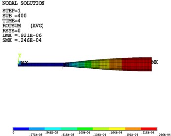
a)
b)
5. Effect of different parameters on response
To take advantage of the superiority of the developed method in effect and accuracy, the studies of the effect of different parametric on the dynamic response are carried out. They are the effect of the impact time of load and the effect of stiffness of the elastic support. Case 4 is taken as shaft model to study the effects of different parameters.
5.1. Effect of impact time of load
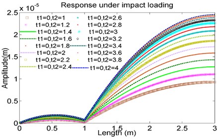
In the study, is same as 0 and the impact time of varies from 1.0 sec to 4.0 sec. The results are given in Fig. 12. As to be expected, increasing the action time, the amplitude of the forced vibration response is increased. It also is observed that there is a quick increase of the amplitude of vibration response occurring at a range of 1secto 3 sec.
Fig. 12The effect of variations of action time t2 on forced vibration response of Case 4
5.2. Effect of stiffness of elastic support
The value of spring stiffness studied is chosen as, namely, 0, 103 N/m, 104 N/m, 105 N/m, 106 N/m, 107 N/m, 108 and 109 N/m, separately. The results are given in Fig. 13.
It can be observed that the forced vibration amplitude of the shaft has a significant increase staring from the 105 N/m. It also can be seen that from the larger the stiffness , the higher is the changing rate of the vibration response amplitude. But as the stiffness is less than 105 N/m or larger than 107 N/m, the vibration response amplitude is constant. That means that in those cases the influence of on vibration response can be negligible. It also can find that in the case 106 N/m, along the shaft axis once over the elastic support the vibration response amplitude is increased and then finally will stay at a constant value. This phenomenon is related to the stiffness property of the elastic supports.
5.3. Effect of location of elastic support
The effect of the location of the elastic supports on vibration response amplitude of the shaft is studied herein. The locations at 0.5 m, 1.5 m, 2 m and 3 m are investigated, separately. The results are given in Fig. 14.
The results show that when the location of the elastic support is closed to the two ends of the shaft, the effects of the elastic support can be negligible and the vibration response amplitude of the shaft is equivalent to that of the shaft with no elastic supports.
From above investigations, the developed method is proved to be an applicable and capable general approach to analysis of the torsional vibration response of shaft with arbitrary boundary conditions, complicated excitation force as well as various elastic supports. Though the examples dealing with are with only an elastic support, as one can be expected, the developed method can be used conveniently to analyze the forced torsional dynamic behaviors for more complicated shaft- elastic support systems in the same way. Another major advantage of the developed method is that, regardless of the number and types of elastic supports, the dynamic equation always can be conveniently established as a single second-order partial differential equation like Eq. (2) which can significantly save the computational effort.
With FEM, when the number of the elastic supports changes, the overall system matrix of the entire structural system has to be rebuilt due to the change of additional freedoms associated with the elastic-support points. However, with the developed method, only a slight change to the overall dynamic equation is required and the process is simple and straightforward. For instance, the effect of the number of elastic supports can be easily reflected in the value in Eq. (2). That is why the developed method is superior over FEM in the computation time and effectiveness.
Fig. 13The effects of variations of the stiffness K on the forced vibration amplitude of Case 4
a)0N/m

b)103 N/m

c)104 N/m
d)105 N/m
e)106 N/m

f)107 N/m
g)108 N/m
h)109 N/m
Fig. 14The effect of the position of the elastic supports on vibration response amplitude of Case 4
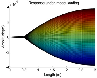
a)107 N/m, 0.5 m
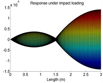
b)107 N/m, 1.5 m
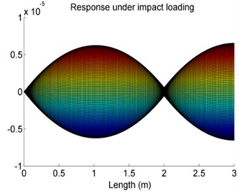
c)107 N/m, 2 m
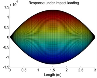
d)107 N/m, 3 m
6. Conclusions
In this paper, an analytical method is developed to solve the torsional forced vibration of a shaft with multiple concentrated inertias and elastic supports under arbitrary boundary conditions based on the two kinds of integral transform methods. The time and the coordinate are carried out the transforms in the Laplace domain and the Fourier domain to obtain the exact solution quickly and accurately, respectively. In comparison with most existing solution procedures for shaft system, such as Eigenfunction Expansion Method and FEM, the results show that this developed method not only is applicable to deal with any boundary conditions, but also can be substantially improved and guaranteed to the speed of solving a complicated shafting model. It is superior over Eigenfunction Expansion Method and FEM in the computation time and effectiveness.
Four cases, the shafts with single concentrated inertia or single elastic support under given boundary conditions, are studied to demonstrate the accuracy and the effectiveness of the developed method. What’s more, the effects of parameters on torsional forced vibration response of shaft are further investigated, including the stiffness and location of elastic supports and the impact time of the loading. The results from the investigation could serve as benchmark solutions for validating new computational techniques in the future.
The developed method successfully provides the exact analytical solution of forced torsional vibration for the shaft with multiple inertias and elastic supports. It can provide a reliable theoretical base not only for analysis and fault diagnosis of a shaft system in engineering signal testing projects but also for the verification of other numerical and analytical methods. Future study will pay attention to extend the developed method to solve other types of vibration problems.
References
-
Qi W. Torsional Vibration of Engine Crankshaft. Qiguang Ying, Shanghai, 2000.
-
Den Hartog J. P., Li J. P. Forced torsional vibrations with damping: an extension of Holzer’s method. Journal of Applied Mechanics, Transactions of ASME, Vol. 68, 1946, p. 276-280.
-
Jong-Shyong W., Wen-Hsiang C. Computer method for forced torsional vibration of propulsive shafting system of marine engine with or without damping. Journal of Ship Research, Vol. 26, Issue 3, 1982, p. 176-189.
-
Doughty S., Vafaee G. Transfer matrix eigensolutions for damped torsional systems. Journal of Vibration, Acoustics, Stress and Reliability in Design, Vol. 107, Issue 1, 1985, p. 128-132.
-
Nengqi X., Ruiping Z., Xiang X., et al. Study on vibration of marine diesel-electric hybrid propulsion system. Mathematical Problems in Engineering, Vol. 2016, 2016, p. 8130246.
-
Ling X., Shixi Y., Chunbiao G. Torsional vibration of a shafting system under electrical disturbances. Shock and Vibration, Vol. 19, Issue 6, 2012, p. 1223-1233.
-
Koibin A. V. Torsional vibration in an elastic rod with external dry friction. Journal of Applied Mathematics and Mechanics, Vol. 58, Issue 5, 1994, p. 941-944.
-
Zhenguo Z., Feng C., Zhiyi Z., Hongxing H. Vibration analysis of non-uniform Timoshenko beams coupled with flexible attachments and multiple discontinuities. International Journal of Mechanical Sciences, Vol. 80, 2014, p. 131-143.
-
Ewing M. S., Mirsafian S. Forced vibration of two beams joined with a non-linear rotational joint: clamped and simply supported end conditions. Journal of Sound and Vibration, Vol. 193, Issue 2, 1996, p. 483-496.
-
Wei J., Tonlo W., W.Kinzy J. The forced vibration of helical springs. International Journal of Mechanical Sciences, Vol. 34, Issue 7, 1992, p. 549-562.
-
Dongying H., Peiming S., Kewei X. Nonlinear torsional vibration dynamics behaviors of rolling Mill’s Multi-DOF main drive system under parametric excitation. Journal of Applied Mathematics, Vol. 2014, 2014, p. 202686.
-
Beytullah T., Faruk Firat C., Naki T. Forced vibration of composite cylindrical helical rods. Journal of Mechanical Sciences, Vol. 47, 2005, p. 998-1022.
-
Bapat C. N., Bhutani N. General Approach for free and forced vibrations of stepped systems governed by the one-dimensional wave equation with non-classical boundary conditions. Journal of Sound and Vibration, Vol. 172, Issue 1, 1994, p. 1-22.
-
Wang H. M., Liu C. B., Ding H. J. Exact solution for forced torsional vibration of finite piezoelectric hollow cylinder. Structural Engineering and Mechanics, Vol. 32, Issue 1, 2009, p. 663-678.
-
Hui L., Zhongchang C., Changle X. Dynamic analysis and multi-object optimization of the forced torsional vibration for vehicular multi-stage planetary gears. Applied Mechanics and Materials, Vol. 86, 2011, p. 263-267.
-
Jaehoon K. Hysterically damped free and forced vibrations of axial and torsional bars by a closed form exact method. Journal of Sound and Vibration, Vol. 378, 2016, p. 144-156.
-
Rudavskii Yu K., Vikovich I. A. Forced flexural-and-torsional vibrations of a cantilever beam of constant cross section. International Applied Mechanics, Vol. 43, Issue 8, 2007, p. 912-923.
-
Sapountzakis E. J. Torsional vibrations of composite bars of variable cross-section by BEM. Computer Methods in Applied Mechanics and Engineering, Vol. 194, Issues 18-20, 2005, p. 2127-2145.
-
Bingen Y. Exact transient vibration of stepped bars, shafts and strings carrying lumped masses. Journal of Sound and Vibration, Vol. 329, 2010, p. 1191-1207.
-
Yuesheng L., Guofeng F., Tao C., et al. Methods of Mathematical Physics. First Edition, National Defense Industry Press, Beijing, 2013.
About this article

This research work was funded by the National Natural Science Foundation of China (Grant No. 51375104), the Heilongjiang Province Funds for Distinguished Young Scientists (Grant No. JC201405), China Postdoctoral Science Foundation (Grant No. 2015M581433), and Postdoctoral Science Foundation of Heilongjiang Province (Grant No. LBH-Z15038).
