Thermal shock behaviour on generalized thermoelastic semi-infinite medium with moving heat source under Green Naghdi-III model

Singh, Biswajit; Pal (Sarkar), Smita

doi:10.21595/mme.2019.20904

Mathematical Models in Engineering

Browse Journal

Submit article

Published: 30 September 2019

Check for updates

Thermal shock behaviour on generalized thermoelastic semi-infinite medium with moving heat source under Green Naghdi-III model

Biswajit Singh¹

Smita Pal (Sarkar)²

^{1, 2}Department of Mathematics, Indian Institute of Engineering Science and Technology (IIEST), Shibpur, Howrah, 711103, West Bengal, India

Corresponding Author:

Biswajit Singh

Cite the article Download PDF

Abstract

The present article deals with the thermal shock response in an isotropic thermoelastic medium with a moving heat source. In this context Green and Naghdi type III model of generalized thermoelasticity theory is considered. The basic equations are expressed as vector-matrix differential equation form. The considered formulation is applied to a semi-infinite solid space. The analytical formulations of the problem in the Laplace transform domain have been solved by eigenvalue approach technique. The inversion of Laplace transform is completed by Zakian method. The variation of the temperature, displacement and stress distributions for different values of time and heat source velocity are shown graphically for two different cases. In the first case, a thermal shock free surface is considered subjected to traction and in the second case the surface is under the influence of time dependent thermal shock. Finally, some comparisons of the results for different time and moving heat source velocity are presented. In presence of moving heat source all the thermophysical quantities have a great significant effect in all the distributions.

Highlights

An eigenvalue approach method is introduced to obtain the analytical expression of the physical quantities of the problem of generalized thermoelasticity with moving heat source.
Significant differences of the displacement component, stress and temperature field are seen for different values time and velocity.
It can be noted that moving heat source velocity has a great expressive effect on the solutions of stress, displacement and temperature field.
From the figures it is clear that the thermal and mechanical boundary conditions is satisfied which indicates that the analytical results agree with numerical results.

1. Introduction

The topic generalized thermoelasticity has increased more consideration of several researchers during last four decades due to its applications in so many fields of applied sciences and mathematics viz. earthquake engineering, nuclear reactor's design, soil dynamics, high energy particle accelerators, etc. The objective of this theory is to succeed in the shortcomings that are inherent in the classical thermoelasticity theory suggested by Biot [1]. In this theory the heat equation is of parabolic type. The infinite speed of thermoelastic disturbance is inherent in that theory and it is unrealistic from physical point of view. To resolve this problem, the classical thermoelasticity theory has been generalized so that a finite speed of thermoelastic disturbance is admitted. In generalized thermoelasticity, the parabolic type heat equation is replaced by hyperbolic type heat equation supported by examinations which display the real existence of wave type heat transportation in solids, known as the second sound effect. The first is because of Cattaneo [2] and Vernotte [3] who proposed generalized version of Fourier’s law to obtain hyperbolic heat conduction equation by introducing a relaxation time, named hereafter C-V model.

The first generalization of the classical theory of thermoelasticity, determined by Lord and Shulman [4], included one relaxation time parameter in Fourier’s law of heat conduction equation. It involved a heat transfer equation of hyperbolic nature declaring finite speed of thermal signals. The temperature-rate-dependent theory (TRDTE) of thermo-elasticity as proposed by Green and Lindsay [5], called G-L theory, involved two relaxation time parameters. This hypothesis achieved a modified variety of the constitutive equations in the coupled theory of thermoelasticty. Suhubi [6] freely found explicit type of constitutive equations. Consequently, a few works [7, 8] based on these generalized models had been examined. Hetnarski and Ignaczak [9] developed low-temperature thermoelasticity dependent on the third generalization of the coupled theory and classified it by a system of non-linear field equations. Heat conduction equation for low-temperature non-linear model estimates that the wave like-thermal signals were supposed to grip at low temperatures. Kosinski et al. [10, 11] had examined Soliton-like waves in a low-temperature non-linear thermoelastic solid. Green and Naghdi [12, 13] formulated the fourth generalization to the theory of coupled thermoelasticity (known as G-N theory) which was concerned without energy dissipation. This theory pursues the Fourier law of heat conduction and proves that heat propagates with finite speed. Chandrasekharaiah et al. [14] had contemplated collaborations with G-N theory without energy dissipation (TEWOED) in an unbounded medium with spherical cavity body. Roy Choudhuri et al. [15] considered propagation of wave with G-N theory without energy dissipation in rotating elastic medium. Numerous problems involving to the G-N theory without energy dissipation other than generalized thermoelasticity were studied [16-19].

Several authors including Gutfield and Netherchot [20], Taylor et al. [21] conducted experiments with various solid bodies and showed that heat pulses do not propagate at infinite speed. He and Cao [22] considered generalized magneto thermoelastic problem subjected to moving heat source. Also, Chandrasekharaiah and Srinath [23] studied the thermolastic interaction without energy dissipation due to a point heat source and line heat source.

Some applications of magneto thermorelasticity using eigenvalue approach technique were examined in the literatures [24, 25]. Das and Bhakata [26] proposed eigenfunction expansion technique to the solution of simultaneous equations and its application in mechanics. Baksi et al. [27] examined magneto-thermoelastic interactions with heat sources and thermal relaxation in a three dimensional unbounded rotating elastic medium. Abbas [28-33]and his colleagues solved different types of problem by eigenvalue approach method which was developed by Das et al. [3] in Laplace transform domain. Baksi et al. [34] and Sinha et al. [35] solved various types of problems considering the effect of rotation and relaxation time in generalized thermoelasticity using eigenvalue approach method. Lahiri et al. [36] used matrix method of solution of coupled differential equation and showed its applications in generalized thermoelasticity.

In this present article, a problem of generalized thermoelasticity subjected to a moving heat source distributed over a plane area in an unbounded isotropic medium is considered. The governing equation of the problem is solved by eigenvalue approach technique developed by Das et al. [38]. The analytical solutions are found for displacement, temperature and stress in the Laplace transform domain. The inversion of Laplace transform has been computed using efficient computer programming. Finally, the resulting quantities to study the effect of the moving heat source for copper material are derived numerically and presented graphically for two different cases.

2. The governing equation

In absence of body force equations of motion take the following form [39]:

1

σ_{i j, j} = ρ {\ddot{u}}_{i} .

The heat conduction is of the form:

2

K^{*} \nabla^{2} T + K \nabla^{2} \dot{T} = \frac{\partial}{\partial t} (ρ c_{e} \dot{T} + γ T_{0} \dot{e} - Q) .

The constitutive equation is given by:

3

σ_{i j} = 2 μ e_{i j} + [λ e - γ (T - T_{0})] δ_{i j} .

Special cases:

If we take $K = 0$ then the problem will be reduced to Green-Naghdi II theory (GN-II).

If we take $K^{*} = 0$ then the problem will be reduced to Green-Naghdi I theory (GN-I).

The displacement u and the temperature field $T$ can be written for one- dimensional problem in the following form: $u = u (x, t)$ , $v = 0$ , $w = 0$ , $T = T (x, t)$ .

Thus Eqs. (1), (2), (3) take the following form:

4

(λ + 2 μ) \frac{\partial^{2} u}{\partial x^{2}} - γ \frac{\partial T}{\partial x} = ρ \frac{\partial^{2} u}{\partial t^{2}},

5

K^{*} \frac{\partial^{2} T}{\partial x^{2}} + K \frac{\partial^{3} T}{\partial t \partial x^{2}} = \frac{\partial}{\partial t} (ρ c_{e} \frac{\partial T}{\partial t} + γ T_{0} \frac{\partial^{2} u}{\partial t \partial x} - Q),

6

σ_{x x} = (λ + 2 μ) \frac{\partial u}{\partial x} - γ (T - T_{0}) .

Introducing the non-dimensional variables:

7

x^{*} = c_{0} η^{'} x, u^{*} = c_{0} η^{'} u, t^{*} = {c_{0}}^{2} η^{'} t,

T^{*} = \frac{γ (T - T_{0})}{(λ + 2 μ)}, σ_{x x}^{*} = \frac{σ_{x x}}{(λ + 2 μ)}, Q^{*} = \frac{γ Q}{K {η'}^{2} ρ {c_{0}}^{4}},

where:

η' = \frac{ρ c_{e}}{K}, c_{0}^{2} = \frac{(λ + 2 μ)}{ρ}, ε_{1} = \frac{K'}{ρ c_{0}^{2} c_{e}}, ε_{2} = \frac{T_{0} γ^{2}}{ρ^{2} c_{0}^{2} c_{e}} .

For simplicity dropping *, Eqs. (4) -(6) take the non-dimensional form as:

8

\frac{\partial^{2} u}{\partial x^{2}} - \frac{\partial T}{\partial x} = \frac{\partial^{2} u}{\partial t^{2}},

9

ε_{1} \frac{\partial^{2} T}{\partial x^{2}} + \frac{\partial^{3} T}{\partial t \partial x^{2}} = \frac{\partial}{\partial t} (\frac{\partial T}{\partial t} + ε_{2} \frac{\partial^{2} u}{\partial t \partial x} - Q),

10

σ_{x x} = \frac{\partial u}{\partial x} - T .

The non-dimensional form of the moving heat source is taken in the following form [40]:

11

Q = Q_{0} δ (x - v t),

where $Q_{0}$ is constant and $δ$ is the delta function and $v$ is the heat source velocity.

3. Initial and boundary conditions

For preceding description, we assume that the medium is initially at rest i.e. at time $t =$ 0, the displacement component and temperature along with their derivatives with respect to t are zero. So the following initial conditions hold:

12

u (x, 0) = \frac{\partial u (x, 0)}{\partial t} = 0, T (x, 0) = \frac{\partial T (x, 0)}{\partial t} = 0 .

Now the boundary conditions at $x = 0$ are taken as.

Case (I):

13

σ = H (t), T = 0, x = 0,

where, $H (t)$ indicates the Heaviside function.

Case (II).

Thermal boundary condition:

T (0, t) = F (t), x = 0 .

Mechanical boundary condition:

14

u (0, t) = 0, x = 0,

where, $F (t) = T^{*} H (t)$ and $T^{*}$ denotes the constant temperature.

4. Laplace transform domains

We define the Laplace transformation on the function $f (t)$ as follows:

15

\bar{f} (s) = L [f (t)] = \int_{0}^{\infty} f (t) e^{- s t} d t .

Applying the Laplace transform under initial conditions to Eqs. (8-10) and (13), (14) we get:

16

\frac{d^{2} \bar{u}}{d x^{2}} - \frac{d \bar{T}}{d x} = s^{2} \bar{u},

17

(ε_{1} + s) \frac{d^{2} \bar{T}}{d x^{2}} = s^{2} \bar{T} + s^{2} ε_{2} \frac{d \bar{u}}{d x} - Q_{0} \frac{s}{v} e^{- \frac{s x}{v}},

18

{\bar{σ}}_{x x} = \frac{d \bar{u}}{d x} - \bar{T},

19

\bar{σ} (0, s) = \frac{1}{s}, \bar{T} (0, s) = 0,

20

\bar{T} (0, s) = T_{0} \frac{1}{s}, \bar{u} (0, s) = 0 .

5. Formulation of the vector- matrix differential equation

The Eqs. (16) and (17) are expressed in the vector-matrix differential form as follows:

21

\frac{d}{d x} [\begin{array}{l} \bar{u} \\ \begin{array}{l} \bar{T} \\ {\bar{u}}^{'} \end{array} \\ {\bar{T}}^{'} \end{array}] = [\begin{matrix} 0 & 0 & 1 & 0 \\ 0 & 0 & 0 & 1 \\ M_{31} & 0 & 0 & M_{34} \\ 0 & M_{42} & M_{43} & 0 \end{matrix}] [\begin{array}{l} \bar{u} \\ \begin{matrix} \bar{T} \\ {\bar{u}}^{'} \end{matrix} \\ {\bar{T}}^{'} \end{array}] + [\begin{matrix} 0 \\ 0 \\ 0 \\ m e^{- s x / v} \end{matrix}],

where:

22

M_{31} = s^{2}, M_{34} = 1, M_{42} = \frac{s^{2}}{ε_{1} + s}, M_{43} = \frac{s^{2} ε_{2}}{ε_{1} + s}, m = \frac{- Q_{0} s}{(ε_{1} + s) v} .

Eq. (21) can be compactly written as:

23

\frac{d \bar{V}}{d x} = \bar{A} (s) \bar{V} + \bar{f},

where:

\bar{A} (s) = [\begin{matrix} 0 & 0 & 1 & 0 \\ 0 & 0 & 0 & 1 \\ M_{31} & 0 & 0 & M_{34} \\ 0 & M_{42} & M_{43} & 0 \end{matrix}], \bar{f} = [\begin{matrix} 0 \\ 0 \\ 0 \\ m e^{- s x / v} \end{matrix}], \bar{V} = [\begin{array}{l} \bar{u} \\ \begin{array}{l} \bar{T} \\ {\bar{u}}^{'} \end{array} \\ {\bar{T}}^{'} \end{array}] .

6. Solution of the vector matrix differential equation

The characteristic equation of the matrix $A$ is given by [38]:

24

η^{4} - (M_{31} + M_{42} + M_{34} M_{43}) η^{2} + M_{31} M_{42} = 0 .

The eigenvalues of the matrix $\bar{A} (s)$ , which are also roots of the characteristic Eq. (24), take the form:

25

η = η_{1}, η = η_{2} = - η_{1}, η = η_{3} = η_{2}, η = η_{4} = - η_{2 .}

The right eigenvector $\vec{X} = {[x_{1}, x {}_{2}, x_{3}, x_{4}]}^{t}$ corresponding to the eigenvalue $η$ can be written as:

26

{[x_{1} = η M_{34}, x_{2} = η^{2} - M_{31}, x_{3} = η^{2} M_{34}, x_{4} = η (η^{2} - M_{31})]}^{t} .

From Eqs. (25) and (26), the eigenvector $X_{i}$ corresponding to the eigenvalue $η = η_{i},$ $i =$ 1, 2, 3, 4 can be easily calculated. The following notations will be used:

27

{\vec{X}}_{1} = {[\vec{X}]}_{η = η_{1}}, {\vec{X}}_{2} = {[\vec{X}]}_{η = - η_{1}}, {\vec{X}}_{3} = {[\vec{X}]}_{η = η_{2}}, {\vec{X}}_{4} = {[\vec{X}]}_{η = - η_{2}} .

Similarly, the left eigenvector $\vec{Y} = [y_{1}, y {}_{2}, y_{3}, y_{4}]$ , corresponding to the eigenvalue $η$ can be calculated as:

28

[y_{1} = \frac{η^{2} - M_{42}}{M_{42}}, y_{2} = \frac{η M_{34}}{M_{31}}, y_{3} = \frac{η (η^{2} - M_{42})}{M_{31} M_{42}}, y_{4} = \frac{η^{2} M_{34}}{M_{31} M_{42}}] .

From Eqs. (25) and (28), we can easily obtain the eigenvector $Y_{i}$ corresponding to the eigenvalue $η = η_{i}$ , $i =$ 1, 2, 3, 4 we use the notation as:

29

{\vec{Y}}_{1} = {[\vec{Y}]}_{η = η_{1}}, {\vec{Y}}_{2} = {[\vec{Y}]}_{η = - η_{1}}, {\vec{Y}}_{3} = {[\vec{Y}]}_{η = η_{2}}, {\vec{Y}}_{4} = {[\vec{Y}]}_{η = - η_{2}} .

Thus, the complementary solution of the Eq. (21) can be written as follows:

30

{\vec{V}}_{c} = \sum_{k = 1}^{4} A_{k} {\vec{X}}_{k} e^{η_{k} x} = A_{2} {[\vec{X}]}_{η = - η_{1}} e^{- η_{1} x} + A_{4} {[\vec{X}]}_{η = - η_{2}} e^{- η_{2} x} .

Since the components of the vector $\vec{V}$ are all finite, when $x \to \infty$ we get $A_{1}$ , $A_{3} \to 0 .$ Therefore, the particular solution ${\vec{V}}_{p}$ should be in the form:

31

{\vec{V}}_{p} = a_{2} (x) {\vec{X}}_{2} e^{- η_{1} x} + a_{4} (x) {\vec{X}}_{4} e^{- η_{2} x}, x > 0,

where:

32

a_{2} (x) = \frac{1}{Y_{2} X_{2}} \int_{- \infty}^{x} Y_{2} \vec{f} (p, s) e^{- η_{1} p} d p = \frac{η_{1}^{2} M_{34} m}{Y_{2} X_{2} M_{31} M_{42} (η_{1} + \frac{s}{v})} [1 - e^{- (η_{1} + \frac{s}{v}) x}], x > 0,

33

a_{4} (x) = \frac{1}{Y_{4} X_{4}} \int_{- \infty}^{x} Y_{4} \vec{f} (p, s) e^{- η_{2} p} d p = \frac{η_{2}^{2} M_{34} m}{Y_{4} X_{4} M_{31} M_{42} (η_{2} + \frac{s}{v})} [1 - e^{- (η_{2} + \frac{s}{v}) x}], x > 0 .

Thus, the general solution of the non-homogeneous system Eq. (23) is:

34

\vec{V} (x, s) = {\vec{V}}_{c} + {\vec{V}}_{p} .

Thus, the expressions of displacement, temperature and stress can be written from Eq. (34) as:

35

\bar{u} (x, s) = - A_{2} M_{34} η_{1} e^{- η_{1} x} - A_{4} M_{34} η_{2} e^{- η_{2} x} - η_{1} a_{2} (x) e^{- η_{1} x} - η_{2} a_{4} (x) e^{- η_{2} x},

36

\bar{T} (x, s) = A_{2} ({η_{1}}^{2} - M_{31}) e^{- η_{1} x} + A_{4} ({η_{2}}^{2} - M_{31}) e^{- η_{2} x}

+ ({η_{1}}^{2} - M_{31}) a_{2} (x) e^{- η_{1} x} + ({η_{2}}^{2} - M_{31}) a_{4} (x) e^{- η_{2} x},

37

{\bar{σ}}_{x x} (x, s) = A_{2} M_{34} η_{1}^{2} e^{- η_{1} x} + A_{4} M_{34} η_{2}^{2} e^{- η_{2} x}

- [\frac{η_{1}^{2} M_{34} m}{Y_{2} X_{2} M_{31} M_{42}} e^{- (η_{1} + \frac{s}{v}) x} + \frac{η_{2}^{2} M_{34} m}{Y_{4} X_{4} M_{31} M_{42}} e^{- (η_{2} + \frac{s}{v}) x}] - \bar{T} (x, s) .

With the help of the boundary conditions, the constants $A_{2}$ , $A_{4}$ can be obtained for case (I) and case (II).

7. Numerical inversion

For the final solution of temperature, displacement and stress distribution in the time domain, the Zakian [37] method for the inversion of Laplace Transform has been applied.

This method $f (t)$ is computed as a sum of weighted evaluations of $F (s)$ :

f (t) = \sum_{i = 1}^{N} K_{i} F (S_{i}),

where the values of $K_{i}$ , $S_{i}$ and $N$ are dictated by a particular method. A significant feature of the derivation is the specification that the time function can be related to a finite series of exponential functions:

\sum_{i = 1}^{N} K_{i} e^{α_{i} t} .

The significance of this specification is that Zakian’s Algorithm is very accurate for overdamped and slightly underdamped systems. But it is not accurate for systems with prolonged oscillations.

Given $F (s)$ and a value of time t, the following equation implements Zakian’s Algorithm and allows us to calculate the numerical value of $f (t)$ :

f (t) = \frac{2}{t} \sum_{i = 1}^{5} R e a l (K_{i} F (\frac{α_{i}}{t})) .

Table 1Values of complex constant for αi and Ki as in [37]

$i$	$α_{i}$	$K_{i}$
1	12.83767675+ $i$ 1.666063445	–36902.0821+ $i$ 196990.426
2	12.22613209+ $i$ 5.012718792	61277.0252– $i$ 95408.6255
3	10.9343031+ $i$ 8.40967312	–28916.5629+ $i$ 18169.1853
4	8.77643472+ $i$ 11.9218539	4655.36114– $i$ 1.90152864
5	5.22545336+ $i$ 15.7295290	–-118.741401– $i$ 141.303691

Zakian’s Algorithm is simple to implement and computes quickly.

8. Numerical results and discussion

For the purpose of numerical simulations, the copper material was chosen, the physical data for which are given in Table 2.

Table 2Material constants

Symbol	Numerical value	Units
$λ$	7.76×10¹⁰	(kg)(m)^-1(s)^-1
$μ$	3.86×10¹⁰	(kg)(m)^-1(s)^-²
$T_{0}$	293	K
$K$	3.86×10²	(kg)(m)(K)^-1(s)^-3
$c_{e}$	3.831×10²	(m)²(K)^-1(s)^-2
$ρ$	8.954×10³	(kg)(m)^-2
$α_{t}$	1.78×10^-6	(K)^-1

The other constants are specified as $Q_{0} =$ 7, $T^{*} =$ 0.6.

Using above data to study the characteristics of displacement, stresses and temperature, we have drawn several figures, Figs. 1-6 for case I and Figs. 7-12 for case II for different values of time and velocity of the moving heat source with distance $x$ , and here the velocity of moving heat source and time has a great effect on all distributions.

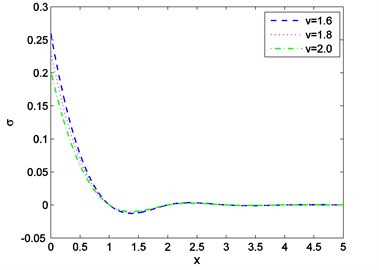
Case-(I): Figs. 1-3 depicts the effect of Temperature ( $T$ ), displacement ( $u$ ) and stress $(σ)$ against distance for different values of time ( $t =$ 0.003, 0.006, 0.009) where velocity of moving heat source, $v =$ 1.5 remains fixed. Figs. 4-6 exhibits the consequence of Temperature ( $T$ ), displacement ( $u$ ) and stress $σ$ with distance for different values of velocity ( $v =$ 1.6, 1.8, 2.0) where ( $t =$ 0.002) remains constant. From Fig. 1 it is seen that magnitude of the temperature decreases with the increase of time and components of temperature obtain its maximum value near $x =$ 0.6 and then it decreases to zero for all values of t. Figs. 2, 4, 5 it is observed that the magnitude of the absolute displacement, absolute temperature increases with the increase of time and velocity. From Fig. 3 we see that absolute value of stress increase with increase of time. Fig. 6 shows that when velocity increases then the magnitude of the stress decreases and stress component will decrease its maximum near $x =$ 2. In all the Figs. 1, 3 and Figs. 4, 6 stress values always initiate from one and end with zero value and magnitude of the temperature starts from zero value and terminate with zero value. These two components also satisfy the physical boundary conditions of the considered problem.

Fig. 1Distribution of temperature against distance for distinct values of t

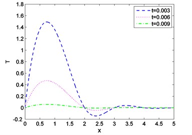
Fig. 2Distribution of displacement against distance for various values of t

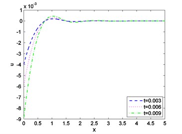
Fig. 3Distribution of stress against distance for various values of t

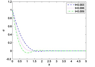
Fig. 4Distribution of temperature against distance for various values of v

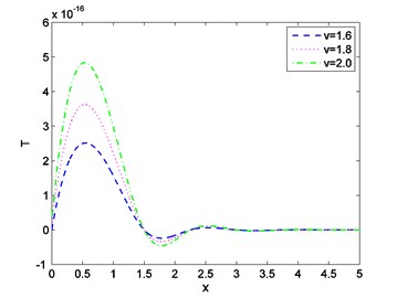
Fig. 5Distribution of displacement against distance for various values of v

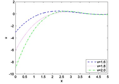
Fig. 6Distribution of stress against distance for various values of v

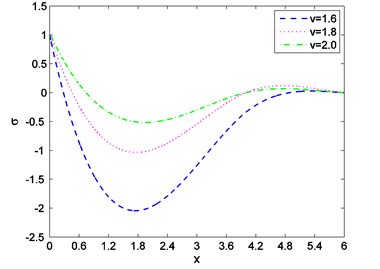
Fig. 7Distribution of temperature against distance for various values of t

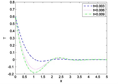
Fig. 8Distribution of displacement against distance for various values of t

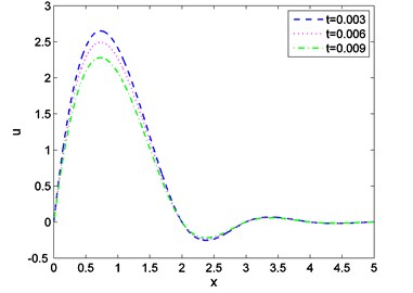
Fig. 9Distribution of stress against distance for various values of t

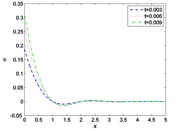
Fig. 10Distribution of temperature against distance for various values of v

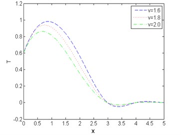
Fig. 11Distribution of displacement with distance for various values of v

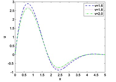
Fig. 12Distribution of stress with distance for various values of v

Case-II: That the absolute value of the temperature distribution increases with increase of time is observed from Fig. 7. Fig. 8 shows that magnitude of displacement decrease with increase of time. From Fig. 9 we observed that distribution of stress increases with the increase of time. From Figs. 10, 11, 12 it is seen that magnitude of displacement, stress and temperature components decrease with increase of velocity of heat source. Finally, all these figures always obey the boundary conditions for this case.

9. Conclusions

In this work, the magnitude of the displacement, temperature and stress have been studied for two cases. In the first case, the surface of the half space $x =$ 0 is subjected to a traction and thermal shock free whereas in the second case, the surface is subjected to a time dependent thermal shock. Analytical expressions for stress, temperature and displacement in the material have been derived. Eigenvalue approach method in Laplace transform domain furnishes good approximation of the solution. It can be noted that moving heat source velocity has a great expressive effect on the solutions of stress, displacement and temperature field.

The results presented in this paper may be helpful for researchers who are working on mathematical physics, mathematical physics, thermodynamics with low temperatures as well as on the development of the hyperbolic thermoelasticity theory.

References

Biot M. A. Thermoelasticity and irreversible thermodynamics. Journal of Applied Physics, Vol. 27, 1956, p. 240-253.

Publisher
Cattaneo C. Sur une former de l’equation de la chaleurelinant le paradoxed’une propagation instance. Comptes Rendus de l’Académie des Sciences, Vol. 247, 1958, p. 431-432.

Search CrossRef
Vernotte M. P. Les paradoxes de la theorie continue de l’equation de la chaleur. Comptes Rendus de l’Académie des Sciences, Vol. 246, 1958, p. 3154-3155.

Search CrossRef
Lord H. W., Shulman Y. A generalized dynamic theory of thermoelasticity. Journal of the Mechanics and Physics of Solids, Vol. 15, 1967, p. 299-309.

Publisher
Green A. E., Lindsay K. A. Thermoelasticity. Journal of Elasticity, Vol. 2, Issue 1, 1972, p. 1-7.

Publisher
Suhubi E. S. Thermoelastic Solids. A. C. Eringen Continuum Physics, Part 2, Academic Press, New York, 1975.

Publisher
Wang J., Dhaliwal R. S., Rokne J. G. Fundamental solutions of the generalized thermo-elastic equations. Journal of Thermal Stresses, Vol. 16, 1993, p. 135-161.

Publisher
Chandrasekharaiah D. S. Wave propagation in thermo-elastic half space. Indian Journal of Pure and Applied Mathematics, Vol. 12, 1981, p. 226-241.

Search CrossRef
Hetnarski R. B., Ignaczak J. Soliton-like waves in a low-temperature non-linear thermoelastic solid. International Journal of Engineering Science, Vol. 34, 1996, p. 1767-1787.

Publisher
Kosinski W. Elastic Waves in the Presence of a New Temperature Scale in Elastic Wave Propagation. Elsevier, New York, 1989, p. 629-634.

Publisher
Kosinski W., Cimmelli V. A. Gradient generalization to inertial state variables and a theory of super fluidity. Journal of Theoretical Applied Mechanics, Vol. 35, 1997, p. 763-779.

Search CrossRef
Green A. E., Naghdi P. M. On undamped heat waves in an elastic solid, Journal of Thermal Stresses, Vol. 15, 1992, p. 253-264.

Publisher
Green A. E., Naghdi P. M. Thermoelasticity without energy dissipation. Journal of Elasticity, Vol. 31, Issue 89, 1993, p. 208-1993.

Search CrossRef
Chandrasekharaiah D. S., Murthy H. N. Thermoelastic interactions in an unbounded body with a special Cavity. Journal of Thermal Stresses, Vol. 16, 1993, p. 55-70.

Publisher
Roy Choudhuri S. K., Bandyopadhyay N. Thermoelastic wave propagation in rotating elastic medium without energy dissipation. International Journal of Mathematics and Mathematical Sciences, Vol. 2005, Issue 1, 2005, p. 99-107.

Publisher
Kumar R., Chawla V. Wave propagation at the boundary surface of elastic layer overlaying a thermoelastic without energy dissipation half-space. Journal of Solid Mechanics, Vol. 2, Issue 4, 2010, p. 363-375.

Search CrossRef
Dhaliwal R. S., Rokne J. G. One-dimensional generalized thermoelastic problem for a half-space. Journal of Thermal Stresses, Vol. 11, 1988, p. 257-271.

Publisher
Chandrasekharaiah D. S., Srinath K. S. One-dimensional waves in a thermoelastic half-space without energy dissipation. International Journal of Engineering Science, Vol. 34, Issue 13, 1996, p. 1447-1455.

Publisher
Abbas I. A. A GN model for thermoelastic interaction in an unbounded fiber-reinforced anisotropic medium with a circular hole. Applied Mathematics Letters, Vol. 26, Issue 2, 2013, p. 232-239.

Publisher
Gutfeld R. J., Nethercot A. H. Temperature dependence of heat- pulse propagation in Sapphire. Physical Review Letters, Vol. 17, 1966, p. 868-871.

Publisher
Taylor B., Maris H. J., Elbaum C. Phonon focusing in solids. Physical Review Letters, Vol. 23, 1969, p. 416-419.

Publisher
Cao L. A problem of generalized magneto-thermoelastic thin slim strip subjected to a moving heat source. Mathematical and Computer Modeling, Vol. 49, Issues 7-8, 2009, p. 1710-1720.

Publisher
Chandrasekharaiah D. S., Srinath K. S. Thermoelastic interactions without energy dissipation due to point heat source. Journal of Elasticity, Vol. 50, Issue 2, 1998, p. 97-108.

Publisher
Das B., Lahiri A. One dimensional generalized magneto thermoelastic problem for a half space. Proceedings of the World Congress on Engineering, 2012.

Search CrossRef
Sarkar N., Lahiri A. Electromagneto thermoelastic interactions in an orthotropic slab with two thermal relaxation times. Computational Mathematics Modelling, Vol. 23, Issue 4, 2012, p. 461-477.

Publisher
Das N. C., Bhakata P. C. Eigen function expansion method to the solution of simultaneous equations and its application in mechanics. Mechanics Research Communications, Vol. 12, 1985, p. 19-29.

Publisher
Baksi A., Bera R. K., Debnath L. A study of magneto-thermoelastic problems with thermal relaxation and heat sources in a three dimensional infinite rotating elastic medium. International Journal of Engineering Science, Vol. 43, Issues 19-20, 2005, p. 1419-1434.

Publisher
Abbas I. A., Abo Dahab S.-M. On the numerical solution of thermal shock problem for generalized magneto thermoelasticity for an infinitely long annular cylinder with variable thermal conductivity. Journal of Computational and Theoretical Nanoscience, Vol. 11, Issue 3, 2014, p. 607-618.

Publisher
Abbas I. A. A GN model based upon two-temperature generalized thermoelastic theory in an unbounded medium with a spherical cavity. Applied Mathematics and Computation, Vol. 245, 2014, p. 108-115.

Publisher
Abas I. A., Abd-Alla, A. N., Othman M. I. A Generalized magneto-thermoelasticity in a fiber- reinforced anisotropic half-space. International Journal of Thermophysics, Vol. 32, Issue 5, 2011, p. 1071-1085.

Publisher
Abbas I. A. Eigenvalue approach for an unbounded medium with a spherical cavity based upon two temperatures generalized thermoelastic theory. Journal of Mechanical Science and Technology, Vol. 28, Issue 10, 2014, p. 4193-4198.

Publisher
Abbas I. A. Eigenvalue approach in three-dimensional generalized thermoelastic interactions with temperature dependent material properties. Computers and Mathematics with Applications, Vol. 68, Issue 12, 2014, p. 2036-2056.

Publisher
Abbas I. A. Generalized magneto thermoelastic interaction in a fiber-reinforced anisotropic hollow cylinder. International Journal of Thermophysics, Vol. 33, Issue 3, 2012, p. 567-579.

Publisher
Baksi A., Bera R. K., Debnath L. Eigenvalue approach the effect of rotation and relaxation time in two dimensional problems of generalized thermoelasticity. International Journal of Engineering Science, Vol. 42, 2004, p. 1573-1585.

Publisher
Sinha M., Bera R. K. Eigenvalue approach the effect of rotation and relaxation time in generalized thermoelasticity. Computers and Mathematics with Applications, Vol. 46, 2003, p. 783-792.

Publisher
Lahiri A., Das N. C., Sarkar S., Das M. Matrix method of solution of coupled differential equations and its application to generalized thermoelasticity. Bulletin of the Calcutta Mathematical Society, Vol. 101, 2009, p. 571-590.

Search CrossRef
Zakian V. Optimization of numerical inversion of Laplace transforms. Electronics Letters, Vol. 6, 1970, p. 667-679.

Search CrossRef
Das N. C., Lahiri A., Giri R. R. Eigenvalue approach to generalized thermoelasticity. Indian Journal of Pure and Applied Mathematics, Vol. 28, Issue 12, 1997, p. 1573-1594.

Search CrossRef
Othman M. I. A., Abbas I. A. Generalized thermoelasticity of Thermal-Shock problem in a non-homogeneous isotropic hollow cylinder with energy dissipation. International Journal of Thermophysics, Vol. 33, Issue 5, 2012, p. 913-923.

Publisher
Tianhu H., Ying G. A one-dimensional thermoelastic problem due to a moving heat source under fractional order theory of thermoelasticity. Advances in Materials Science and Engineering, Vol. 2014, 2014, p. 510205.

Search CrossRef

Cited by

Photo-thermoelastic behavior of a functionally graded? Semiconductor medium excited by thermal laser pulses

E Awwad | Ahmed E Abouelregal | Doaa Atta | Hamid M Sedighi

(2022)

Magneto-thermoelastic interaction with memory response due to laser pulse under Green-Naghdi theory in an orthotropic medium

Biswajit Singh | Smita Pal (Sarkar)

(2022)

Memory response in dual-phase-lag thermoelastic medium due to instantaneous heat source

Saroj Mandal | Biswajit Singh | Smita Pal(Sarkar)

(2022)

Magneto-thermoelastic interaction in transversely isotropic medium with memory dependent derivative under three theories

Biswajit Singh | Smita Pal (Sarkar)

(2022)

State–space approach on two-temperature three-phase-lag thermoelastic medium with a spherical cavity due to memory-dependent derivative

Biswajit Singh | Smita Pal Sarkar

(2021)

Eigenfunction approach to generalized thermo-viscoelasticity with memory dependent derivative due to three-phase-lag heat transfer

Biswajit Singh | Smita Pal (Sarkar) | Krishnendu Barman

(2020)

Temperature-Rate-Dependent Thermoelasticity Theory With Memory-Dependent Derivative: Energy, Uniqueness Theorems, and Variational Principle

Biswajit Singh | Indranil Sarkar | Smita Pal (Sarkar)

(2020)

Analysis of a functionally graded thermopiezoelectric finite rod excited by a moving heat source

Ahmed E. Abouelregal | Shao-Wen Yao | Hijaz Ahmad

(2020)

About this article

Received

14 July 2019

Accepted

21 August 2019

Published

30 September 2019

DOI

https://doi.org/10.21595/mme.2019.20904

Keywords

generalized thermoelasticity

eigenvalue approach

Laplace transform

vector-matrix differential equation

This is an open access article distributed under the Creative Commons Attribution License, which permits unrestricted use, distribution, and reproduction in any medium, provided the original work is properly cited.

Previous article in issue Previous Next article in issue Next

Research article

2023 06 26

Influence of the fractional-order strain on an infinite material with a spherical cavity under Green-Naghdi hyperbolic two-temperature thermoelasticity theory

Hamdy M. Youssef, Abdulrahman A. Alghamdi

Research article

2021 09 13

Hyperbolic two-temperature generalized thermoelasticity with fractional order strain of solid cylinder

Alaa A. El-Bary

Research article

2017 06 30

Dynamic problem in 3D thermoelastic half-space with rotation in context of G-N type II and type III

S. Santra, A. Lahiri, N. C. Das

Research article

2017 06 30

Two-dimensional generalized thermo-elastic problem for anisotropic half-space

Debkumar Ghosh, Abhijit Lahiri, Ibrahim A. Abbas

B. Singh and S. Pal (Sarkar), “Thermal shock behaviour on generalized thermoelastic semi-infinite medium with moving heat source under Green Naghdi-III model,” Mathematical Models in Engineering, Vol. 5, No. 3, pp. 79–89, Sep. 2019, https://doi.org/10.21595/mme.2019.20904

Copy Extrica

Copied to clipboard!

TY  - JOUR
DO  - 10.21595/mme.2019.20904
UR  - https://doi.org/10.21595/mme.2019.20904
TI  - Thermal shock behaviour on generalized thermoelastic semi-infinite medium with moving heat source under Green Naghdi-III model
T2  - Mathematical Models in Engineering
AU  - Singh, Biswajit
AU  - Pal (Sarkar), Smita
PY  - 2019
DA  - 2019/09/30
PB  - JVE International Ltd.
SP  - 79-89
IS  - 3
VL  - 5
SN  - 2351-5279
SN  - 2424-4627
ER  - 

Copy Ris

Copied to clipboard!

@article{Singh_2019,
	doi = {10.21595/mme.2019.20904},
	url = {https://doi.org/10.21595/mme.2019.20904},
	year = 2019,
	month = {sep},
	publisher = {{JVE} International Ltd.},
	volume = {5},
	number = {3},
	pages = {79--89},
	author = {Biswajit Singh and Smita Pal (Sarkar)},
	title = {Thermal shock behaviour on generalized thermoelastic semi-infinite medium with moving heat source under Green Naghdi-{III} model},
	journal = {Mathematical Models in Engineering}
}

Copy Bibtex

Copied to clipboard!

[1]B. Singh and S. Pal (Sarkar), “Thermal shock behaviour on generalized thermoelastic semi-infinite medium with moving heat source under Green Naghdi-III model,” Mathematical Models in Engineering, vol. 5, no. 3, pp. 79–89, Sep. 2019, doi: 10.21595/mme.2019.20904.

Copy IEEE

Copied to clipboard!

Singh, Biswajit, and Smita Pal (Sarkar). “Thermal Shock Behaviour on Generalized Thermoelastic Semi-Infinite Medium with Moving Heat Source under Green Naghdi-III Model.” Mathematical Models in Engineering 5, no. 3 (September 30, 2019): 79–89. https://doi.org/10.21595/mme.2019.20904.

Copy Chicago

Copied to clipboard!

Thermal shock behaviour on generalized thermoelastic semi-infinite medium with moving heat source under Green Naghdi-III model

Abstract

Highlights

1. Introduction

2. The governing equation

3. Initial and boundary conditions

4. Laplace transform domains

5. Formulation of the vector- matrix differential equation

6. Solution of the vector matrix differential equation

7. Numerical inversion

8. Numerical results and discussion

9. Conclusions

References

Cited by

About this article

Related Articles