Mathematical model of the vibration cone crusher with three degrees of freedom

Morozov, Petr; Miheev, Serge

doi:10.21595/vp.2019.20790

Vibroengineering Procedia

Browse Procedia

Published: 25 June 2019

Check for updates

Mathematical model of the vibration cone crusher with three degrees of freedom

Petr Morozov¹

Serge Miheev²

¹Mekhanobr-Tekhnika, St. Petersburg, Russia

²St. Petersburg State University, St. Petersburg, Russia

Corresponding Author:

Petr Morozov

Cite the article Download PDF

Downloads 1778

CrossRef Citations 2

Abstract

The project of the vibration crusher with three degrees of freedom is proposed. The degrees are limited by the guide rails that hold the crusher body and cone against horizontal and spiral motions. The mathematical model for this project is obtained. The observations for the motion of the body, the cone and the unbalance vibrator are made in a numerical experiment. A fourfold superiority of the cone amplitude over the body amplitude was discovered. When the cone partial frequency exceeds the unbalance rotation frequency, a strongly marked beating in the cone oscillations was observed with a frequency 8 times less than the unbalance rotation frequency. At the same frequencies, a body beating was observed.

1. Introduction

In modern productions, when crushing solid materials, vibration cone crushers are very promising for use, as the principles of the material optimal crushing are most fully implemented here [1-4]. A greater number of degrees of freedom in vibration crushers predetermines, of course, a greater motion variety [5]. But then the problems of crushing quality become difficult to solve analytically, and they require extensive experiments to determine the optimal crusher parameters. Indeed, estimation about the influence of “swinging”, horizontal and spiral cone motions on crushing can be found out only after the analysis of a real installation with real material, and observation of many parameters. A priori, it can be only assumed that swinging and horizontal displacements lead to increase energy costs, as well as reduce the quality of the crushed material.

Leaving the question of the spiral motion advantage open, note that it is possible to get rid of all three ones constructively, allowing the body and the cone to move only vertically. Besides their elimination, this allows to work with one unbalance vibrator instead of a pair.

The mathematical model for the suggested project differs a lot from the models of vibration crushers with a greater number of degrees of freedom.

2. Main text

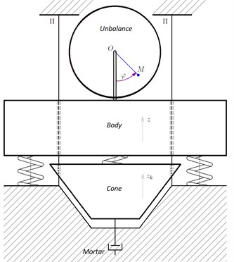
The crusher with three degrees of freedom contains 3 moving parts. The body fixed to the base with spiral springs. The crushing cone connected to the body with spiral springs. And the unbalance installed in the bearings of the crusher body. The unbalance rotates around its own horizontal axis $O$ in the bearings. The unbalance is set in motion by the standing on the base asynchronous electric engine through an elastic coupling. The body and the cone can only move vertically along the guides $Π$ . That is, the body and the cone make straight vertical oscillations along the guides $Π$ (Fig. 1).

At idling, the friction in the unbalance bearings is negligible compared to the friction of the body and the cone on the guides. In the work mode, the friction in the bearings and the friction on the guides can be neglected compared to the resistance beneath the cone, taking into account the presence of destructible material in the crushing chamber.

Note that the small friction between the body and the guides can be provided technically by eliminating lateral loads from the unbalance. In this case, the mathematical model will be identical to the model with a single unbalance vibrator. Then the difference will be only in the friction coefficient.

Fig. 1A general scheme of a vibration cone crusher

The equations describing the motion of the body and the cone are simple enough, and the equations for the unbalance are rather cumbersome.

Let a fixed rectangular Cartesian coordinate system be as follows. Assign a point on the axis $O$ at time 0 as the origin of the coordinates $\vec{0}$ of the system. The “zero” $\vec{0}$ of the system is placed in a certain point on the axis $O$ at time 0. The axes $x$ and $z$ are the perpendiculars to the axis $O$ through $\vec{0}$ chosen in the following way. The $z$ axis is vertically up; the $x$ axis is horizontal from left to right. The rotation axis $O$ at time 0 obviously coincides with the axis $y$ , which does not participate in the description of the considered flat-parallel motion. The unbalance center of mass is denoted by $M$ , $r ≔ |O M|$ . The unbalance phase is the angle $φ$ from the lower $z$ semi-axis counterclockwise to the ray from $O$ to $M$ .

If the masses of the unbalance, the body and the cone are denoted by $m_{D}$ , $m_{b}$ and $m_{k}$ , respectively, then the rotation axis $O$ moves with acceleration with the vertical component ${\ddot{z}}_{M}$ and the horizontal component ${\ddot{x}}_{M}$ . Then the unbalance mass inertia force has a vertical component $F$ and a horizontal component $f$ that satisfy the equations:

\{\begin{array}{l} m_{D} {\ddot{z}}_{M} = F + P, \\ m_{D} {\ddot{x}}_{M} = f, \end{array}

where $P = m_{D} g$ is the unbalance weight.

The angular acceleration is determined by the moments of forces $F$ and $f$ relative to the unbalance gravity center $M$ , and by the asynchronous electric engine moment of force proportional to the difference of the unbalance angular velocity $\dot{φ}$ and the magnetic field angular velocity $ω$ :

1

I \ddot{φ} = μ (ω - \dot{φ}) - F r \sin φ - f r \cos φ,

where $I$ is the unbalance inertia moment, $μ$ is some coefficient.

The transversal acceleration module of the axis $O$ with respect to $M$ is $\ddot{u} ≔ |\ddot{φ}| r$ , and the radial acceleration module of the axis $O$ with respect to $M$ is $\ddot{v} ≔ {\dot{φ}}^{2} r$ . The directions of these accelerations are shown in Fig. 2.

Fig. 2The unbalance dynamic scheme

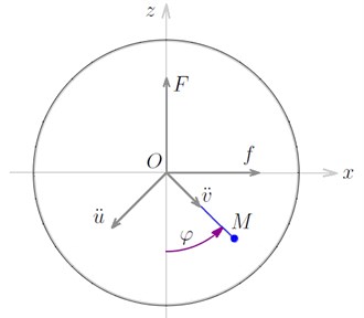
From here, the horizontal axis acceleration is obtained analytically according to the connection:

2

0 = \ddot{x} = {\ddot{x}}_{M} - \ddot{u} \cos φ + \ddot{v} \sin φ = \frac{f}{m_{D}} - \ddot{φ} r \cos φ + {\dot{φ}}^{2} r \sin φ

= \frac{f}{m_{D}} - \frac{μ (ω - \dot{φ}) - F r \sin φ}{I} r \cos φ + \frac{f r^{2} \cos^{2} φ}{I} + {\dot{φ}}^{2} r \sin φ \Rightarrow

3

f = \frac{(μ (ω - \dot{φ}) - F r \sin φ) r \cos φ - I {\dot{φ}}^{2} r \sin φ}{\frac{I}{m_{D}} + r^{2} \cos^{2} φ},

and vertical axis acceleration equal to body acceleration:

4

\ddot{z} = {\ddot{z}}_{M} - \ddot{u} \sin φ - \ddot{v} \cos φ = \frac{F + P}{m_{D}} - \ddot{φ} r \sin φ - {\dot{φ}}^{2} r \cos φ .

In addition, there are two more equations for the body and the cone. Let $z$ and $z_{k}$ be the vertical deviations of any point of the body and any point of the cone from their equilibrium positions, respectively. Such parameters allow to describe the body and cone accelerations without attracting gravity:

5

m_{b} \ddot{z} = κ (z_{k} - z) - κ^{'} z - F,

6

m_{k} {\ddot{z}}_{k} = κ (z - z_{k}) - τ {\dot{z}}_{k},

where $κ$ and $κ^{'}$ are the effective stiffness coefficients of the springs that connect the body with the cone and the body with the base, respectively. The term $τ {\dot{z}}_{k}$ is an approximate model of crushing, and is destined for further discussion. At idle, this model rather adequately describes the cone friction on the guides.

Eqs. (2)-(4) yield:

\ddot{z} \cos φ = \frac{(F + P) \cos φ - f \sin φ}{m_{D}} - {\dot{φ}}^{2} r

= \frac{(F + P) \cos φ}{m_{D}} + \frac{(F r \sin^{2} φ - μ (ω - \dot{φ}) \sin φ) r \cos φ + I {\dot{φ}}^{2} r \sin^{2} φ}{I + m_{D} r^{2} \cos^{2} φ} - {\dot{φ}}^{2} r

= (\frac{P}{m_{D}} + \frac{(F r \sin^{2} φ - μ (ω - \dot{φ}) \sin φ) r \cos φ + I {\dot{φ}}^{2} r \sin^{2} φ}{I + m_{D} r^{2} \cos^{2} φ}) \cos φ .

Hence:

\ddot{z} = {(1 + \frac{m_{b} (\frac{I}{m_{D}} + r^{2})}{I + m_{D} r^{2} \cos^{2} φ})}^{- 1} g

+ \frac{(κ (z_{k} - z) - κ' z) (\frac{I}{m_{D}} + r^{2}) - μ (ω - \dot{φ}) r \sin φ - {\dot{φ}}^{2} r \cos φ (I + m_{D} r^{2})}{I + m_{D} r^{2} \cos^{2} φ + m_{b} (\frac{I}{m_{D}} + r^{2})} .

The value $J ≔ I + m_{D} r^{2}$ is the unbalance inertia moment with respect to the axis $O$ . It yields:

7

\ddot{z} = \frac{J - m_{D} r^{2} \sin^{2} φ}{J (1 + \frac{m_{b}}{m_{D}}) - m_{D} r^{2} \sin^{2} φ} g

+ \frac{(κ (z_{k} - z) - κ' z) \frac{J}{m_{D}} - μ (ω - \dot{φ}) r \sin φ - {\dot{φ}}^{2} J r \cos φ}{I + m_{D} r^{2} \cos^{2} φ + m_{b} (\frac{I}{m_{D}} + r^{2})} .

The Eq. (1) is transformed by taking $J$ and Eq. (3) into account:

\ddot{φ} = μ (ω - \dot{φ}) - (F r \sin φ + \frac{(μ (ω - \dot{φ}) - F r \sin φ) r \cos φ - I {\dot{φ}}^{2} r \sin φ}{\frac{I}{m_{D}} + r^{2} \cos^{2} φ} r \cos φ)

= μ (ω - \dot{φ}) - (F r \sin φ (\frac{I / m_{D}}{I / m_{D} + r^{2} \cos^{2} φ})

+ \frac{(μ (ω - \dot{φ}) \cos φ - I {\dot{φ}}^{2} \sin φ) r^{2} \cos φ}{\frac{I}{m_{D}} + r^{2} \cos^{2} φ})

= I \cdot \frac{μ (ω - \dot{φ}) - F r \sin φ + {\dot{φ}}^{2} m_{D} r^{2} \sin φ \cos φ}{J - m_{D} r^{2} \sin^{2} φ} .

Taking into account $F = κ (z_{k} - z) - κ^{'} z - m_{b} \ddot{z}$ leads to:

8

\ddot{φ} = \frac{μ (ω - \dot{φ}) - F r \sin φ + {\dot{φ}}^{2} m_{D} r^{2} \sin φ \cos φ}{J - m_{D} r^{2} \sin^{2} φ} .

So, in addition to Eqs. (6)-(8), there is one more connection:

9

f = \frac{(μ (ω - \dot{φ}) - F r \sin φ) r \cos φ - I {\dot{φ}}^{2} r \sin φ}{\frac{I}{m_{D}} + r^{2} \cos^{2} φ} .

Solving Eqs. (6)-(8) analytically is difficult. Therefore, they are researched with numerical methods. The time for reaching the stationary mode and the amplitude of the body and the cone oscillations in it for different values of $ω$ and $τ$ are of interest.

There have been assigned $m_{b} ≔$ 59 kg, $m_{k} ≔$ 7.4 kg, $m_{D} ≔$ 2.02 kg, $κ ≔$ 12000 N/m, $κ' ≔$ 12000∙7 N/m, $ω \in$ (0, 160) rad/s.

According to the unbalance geometry, its inertia moment is calculated $I ≔$ 0.295 kg∙m².

Thus, the partial frequency of cone natural oscillations without friction is $\sqrt{κ^{'} / m_{k}} \approx$ 127.9 rad/s. The partial frequency of body natural oscillations with the fixed cone is the same. The unbalance rotation at resonant frequencies is of interest. That is, about 20 rev/sec = 1200 rev/min. This corresponds to a somewhat higher rotational speed of the stator magnetic field, which is included into the considered range.

3. Results

Numerical integration made it possible to obtain graphical dependences of body and cone motions on time, frequency $ω$ and slip friction coefficient $τ$ .

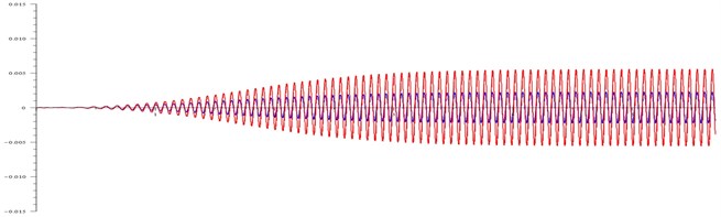
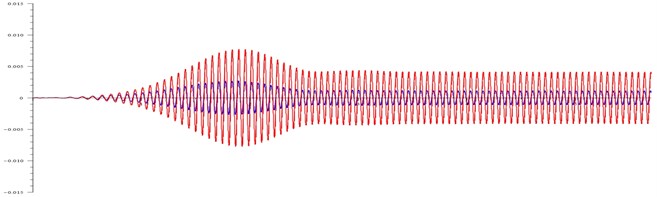
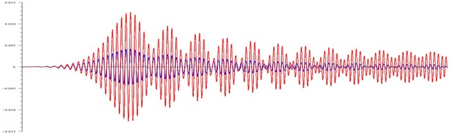
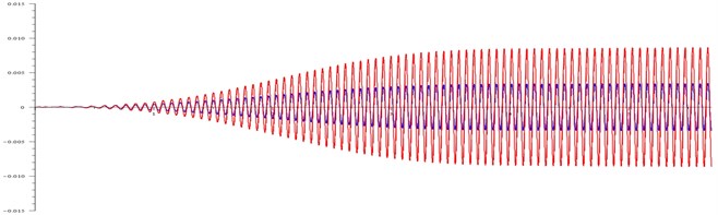
Fig. 3Displacement (in meters) of the body and the cone at: a) ω= 99 rad/ s and τ= 100, b) ω= 110 rad/ s and τ= 100, c) ω= 120 rad/ s and τ= 20, d) ω= 120 rad/ s and τ= 20

a)

b)

c)

d)

As can be seen in Fig. 3(a), when the rotation frequency of the magnetic field is close to resonant, the friction $τ$ is large, the beating is absent both on the body and on the cone, the amplitude of the cone reaches maximum values, which essentially determines the resonance.

As can be seen in Fig. 3(b), the rotation frequency of the magnetic field slightly exceeds the cone resonance frequency. During the acceleration of the rotor, it passes the resonant frequency. Therefore, at this time the oscillation amplitudes of the cone and the body reach maximum values.

As can be seen in Fig. 3(c), the relatively small friction $τ =$ 20 gives “beating” at the magnetic field rotation frequencies that exceed the resonant ones. The body beats are hardly noticeable, and the cone amplitude changes twice.

As can be seen in Fig. 3(d), with a tenfold friction decrease, the resonance view is the same as with high friction. The only difference is that its value reaches 0.009 m instead of 0.005 m with high friction.

4. Conclusions

Numerical experiments showed that the crusher behaves in the classical way in a situation with a resonance. That is, a gradual amplitude increase of the oscillations with an exit to some stable state with the maximum amplitude of the oscillations. At the same time, it has interesting motion features of crusher parts when the rotation frequency of the magnetic field exceeds the resonant one.

While the cone and the body have oscillations that are close in shape to the sum of two sinusoidal oscillations (Fig. 1) with close frequencies and their total period $T$ is approximately 8 times greater than the two oscillations have got, i.e. the mass ratio of the body and the cone. That is, $α_{1} = n / A$ and $α_{1} = (n + 1) / A$ , where $n$ is natural, $A \approx$ 8, $n / A \approx$ 28 rad/s. In this case, in the cone, the amplitude of one harmonic was 25 % of the amplitude of the other. In the body, the amplitude of one harmonic was 10 % of the amplitude of the other.

The constructive elimination of “swinging”, horizontal and spiral motions of the body and the cone opens up access to the modeling of the crushing process using delta functions, which can be integrated in the form of a simple saltatory decrease in the cone speed [6]. Also, perhaps more important, it opens the way for operational optimization of the crushing mode through the rotation frequency control of the stator magnetic field [7].

References

Chanturiya V. A., Vaisberg L. A., Kozlov A. P. Priority research areas in mineral processing. Journal Obogashchenie Rud, Vol. 2, 2014, p. 3-9.

Publisher
Vaisberg L. A., Zarogatsky Turkin L. P. V. Y. Vibratory Crushers. Basis for Calculation, Design Engineering and Industrial Application. VSEGEI, St. Petersburg, 2004.

Search CrossRef
Revnivtsev V. I. On the rational organization of minerals release in accordance with modern outlooks of solid state physics. Vol. 140, Trudy Mekhanobra, Leningrad, 1975, (in Russian).

Search CrossRef
Vaisberg L. A., Zarogatsky L. P. New generation of jaw and cone crushers. Journal Building and Road Construction Machinery, Vol. 7, 2000, p. 16-21.

Search CrossRef
Shishkin E. V., Kazakov S. V. Vibratory crusher forced oscillations in resonance frequency range. Journal Obogashchenie Rud, Vol. 5, 2015, p. 42-45.

Publisher
Trubetskov D. I., Rozhnev A. G. Linear Oscillations and Waves. Fizmatlit, Moscow, 2001.

Search CrossRef
Dikusar V. V., Zubov A. V., Zubov N. V. Structural minimization of stationary control and observation systems. Journal of Computer and Systems Sciences International, Vol. 49, Issue 4, 2010, p. 524-528.

Publisher

Cited by

Stability and Control Processes

Serge E. Miheev | Petr D. Morozov

(2022)

Stochastic model of the stroke of a two-mass cone crusher

Petr Morozov | Serge Miheev

(2020)

About this article

Received

10 May 2019

Accepted

03 June 2019

Published

25 June 2019

SUBJECTS

Mechanical vibrations and applications

DOI

https://doi.org/10.21595/vp.2019.20790

Keywords

vibration crusher

inertial unbalance vibrator

forced oscillations

resonant frequencies

resonant amplitudes

stationary mode

Acknowledgements

Financial support was provided by the Russian Science Foundation No. 17-79-30056 (Project REC “Mekhanobr-tekhnika”).

This is an open access article distributed under the Creative Commons Attribution License, which permits unrestricted use, distribution, and reproduction in any medium, provided the original work is properly cited.

Previous article in issue Previous Next article in issue Next

Research article

2021 09 21

Creation and verification of spatial mathematical model of vibrating machine with two self-synchronizing unbalanced exciters

Ilya Lyan, Grigory Panovko, Alexander Shokhin

Research article

2021 09 03

Dynamics features of a resonant vibromachine with self-synchronizing inertial vibroexciters in the presence of vibration limiter

Grigory Panovko, Alexander Shokhin

Research article

2020 06 29

Slow oscillations in systems with inertial vibration exciters

Nikolay Yaroshevich, Vitalii Puts, Тetjana Yaroshevich, Oleksandr Herasymchuk

Research article

2020 06 29

Stochastic model of the stroke of a two-mass cone crusher

Petr Morozov, Serge Miheev

P. Morozov and S. Miheev, “Mathematical model of the vibration cone crusher with three degrees of freedom,” Vibroengineering PROCEDIA, Vol. 25, pp. 42–47, Jun. 2019, https://doi.org/10.21595/vp.2019.20790

Copy Extrica

Copied to clipboard!

TY  - JOUR
DO  - 10.21595/vp.2019.20790
UR  - https://doi.org/10.21595/vp.2019.20790
TI  - Mathematical model of the vibration cone crusher with three degrees of freedom
T2  - Vibroengineering PROCEDIA
AU  - Morozov, Petr
AU  - Miheev, Serge
PY  - 2019
DA  - 2019/06/25
PB  - JVE International Ltd.
SP  - 42-47
VL  - 25
SN  - 2345-0533
SN  - 2538-8479
ER  - 

Copy Ris

Copied to clipboard!

@article{Morozov_2019,
	doi = {10.21595/vp.2019.20790},
	url = {https://doi.org/10.21595/vp.2019.20790},
	year = 2019,
	month = {jun},
	publisher = {{JVE} International Ltd.},
	volume = {25},
	pages = {42--47},
	author = {Petr Morozov and Serge Miheev},
	title = {Mathematical model of the vibration cone crusher with three degrees of freedom},
	journal = {Vibroengineering {PROCEDIA}}
}

Copy Bibtex

Copied to clipboard!

[1]P. Morozov and S. Miheev, “Mathematical model of the vibration cone crusher with three degrees of freedom,” Vibroengineering PROCEDIA, vol. 25, pp. 42–47, Jun. 2019, doi: 10.21595/vp.2019.20790.

Copy IEEE

Copied to clipboard!

Morozov, Petr, and Serge Miheev. “Mathematical Model of the Vibration Cone Crusher with Three Degrees of Freedom.” Vibroengineering PROCEDIA 25 (June 25, 2019): 42–47. https://doi.org/10.21595/vp.2019.20790.

Copy Chicago

Copied to clipboard!

Mathematical model of the vibration cone crusher with three degrees of freedom

Abstract

1. Introduction

2. Main text

3. Results

4. Conclusions

References

Cited by

About this article

Related Articles