Abstract
A fair evaluation of an electrolytic capacitor time to failure is important for the design and development of electronic devices. In practice, it is required to consider variable operating conditions, for example, weather temperature fluctuations or load variations. Based on the principle of Miner’s fatigue accumulation and reasonable approximations, the general formulas are derived that take into account weather temperature changes. The outdoor air temperature was modeled by the sum of components like averaged seasonal changes, averaged daily temperature changes and random temperature fluctuations. An Easy-to-use analytical formulas for the electrolytic capacitor life time estimation were obtained, in which the contribution of each individual temperature phenomenon can be evaluated. The impact of these components on the non-linear estimation formula by the Miner's principle has been clarified for some example climatic regions. Also, the capacitor life time estimation formula under particularly scheduled variable load was derived for example. The resulting formulas are useful for engineering calculations of the reliability of electronic devices exposed to weather temperature changes.
1. Introduction
Electrolytic capacitors are widely used in a variety of electronics application as indispensable energy temporary storages, but they are the most critical components in terms of limited service time [1-4]. An electrolytic capacitor is a complex electrochemical device whose reliability is influenced by various factors such as voltage, current, frequency, and environment: temperature, humidity, etc. The prediction of the service life of capacitors is the subject of ongoing research. For engineering calculations it is very important to be able to quantitatively evaluate acceptable service time of a capacitor. Extensive empirical data [5-9] suggest that degradation processes are characterized by a strong dependence on temperature according to the semi-empirical Arrhenius law known from chemistry. With a capacitor temperature increase by 10 °C, it’s operating time is halved according to Eq. (1):
where – is the mean time to failure, is the current temperature, – is the time to failure during operation at the nominal temperature . The kind of Arrhenius law stated by the Eq. (1) is generally accepted for use. Capacitor manufacturers provide product designers with their brand life time estimation formulas that do not differ much from Eq. (1) [13-16]. The peculiarity is that the constant is found from experimental data for standard conditions and is provided in specifications for designers to refine calculations in a particular application. In the scientific literature [8, 9] more complex formulas are proposed that take into account the dependence of a capacitor operating time on voltage, frequency and humidity of the environment. The critical factors were taken into account by expanding of expression for in Eq. (1) with corresponding multipliers. Those formulas including Eq. (1) are generalized statistical formulas valid for constant factors throughout the life cycle of a capacitor and take well into account the main degradation mechanism – the capacitor electrolyte evaporation, which is a temperature sensitive process. Of course, most devices do not work around the clock under constant external conditions. More commonly, many electronic devices operate under scheduled load or outdoor, where they are prone to temperature extremes. Therefore, it would be useful to obtain an estimate of the capacitor operating time and possibly the entire electrical device in a variable mode of operation. For this, the analogy with the Miner’s principle of fatigue accumulation [10] have been exploited in [11] to get modified Eq. (2) for capacitors life time :
It is supposed that in Eq. (2) – is the time to failure, known for a product series under constant operating conditions – , , , etc. And is the same found by static expressions in Eq. (1). It is obvious that the Eq. (2) is correct under slowly changing operating conditions, when the capacitor passes through equilibrium steady-state conditions.
Conventional methods include numerical calculations of life time integral of Eq. (2). It is quiet complicated to estimate electrolytic capacitor life time with the help of Eq. (2) without simplifying dynamic models for instantaneous input data massive like outdoor air temperature. Therefore, in some methods like in [11, 12] variable external conditions were often modeled with time intervals , during which affecting degradation factors are considered to be constant. With this assumption one can get from Eq. (2) the Eq. (3):
where is the resulting operating time under alternating mode conditions, is the time fraction during which degradation factors are constant, is the would be operating time if the th mode was valid all the time . For example in the work [12] a capacitor life time was calculated under weather temperature changes, where only averaged over years slowly changing seasonal temperature have been taken into account and further approximated with a limited number of time intervals, during which the temperature is considered to be constant, hence the time to failure was calculated by the Eq. (3). In Eq. (3) daily temperature changes were not possible to consider due to the data size to be processed. Therefore in [12] the influence of daily temperature oscillations was not considered and was remained obscure, not to mention random temperature fluctuations. It will not be correct if one estimates in Eq. (2), substituting averaged factor’s values instead of instantaneous values, because fluctuations around averaged values will have biasing effect on the non-linear Eq. (2).
In the current work electrolytic capacitor life time evaluation formulas have been proposed, which take into account seasonal and daily temperature changes. And more, random temperatures fluctuations around averaged data have been considered also. An easy-to-use formula for electrolytic capacitor life time estimation was obtained, in which the contribution of each individual temperature phenomenon is clear. The life time correction coefficients corresponding to the average seasonal changes, the average daily changes and random temperature fluctuations have been calculated for some climatic regions to evaluate the contribution of each temperature phenomena. Also, the capacitor life time estimation formula under particularly scheduled variable load was derived.
2. Outdoor air temperature model
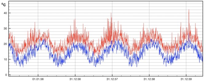
To calculate a capacitor life time one should have fair knowledge of the future instantaneous external temperature , or take historical data and extrapolate them into the future. In this paper the model was proposed to avoid dealing with huge amount of instantaneous weather temperature values. For example, on Fig. 1 daily temperature data over 1955-1960 years for Sydney Observation Hill in Australia is presented [17], where seasonal temperature waves can clearly be distinguished with yearly periodicity. The whole picture on Fig. 1 can be seen as a sum of the average seasonal oscillation and distorting temperature fluctuations. The difference between daily maximums and minimums could seem constant if it got rid of fluctuations. Therefore, let us represent instantaneous air temperature as:
where and are periodic functions corresponding to averaged year and daily periodic oscillations. absorbs all possible errors between real instantaneous temperature values and modeled average curve. It can be attributed to deviations causes by small scale events like clouds, wind gusts, shadows, rains, as well as large scale events like moving weather fronts.
Fig. 1Daily temperature data for Sydney Observation Hill, 1955y-1960y. Red line – daily maximum, blue line – daily minimum. Australian Bureau of Meteorology (BOM)
2.1. Seasonal temperature model
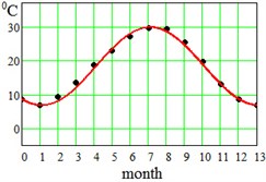
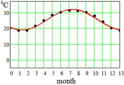
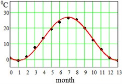
Weather recording services provide with some few major data on air temperature, solar irradiance and humidity [18-29]. On Table 1 there are air temperature statistical data presented for some localities. The data on Table 1 can be approximated by the harmonic function:
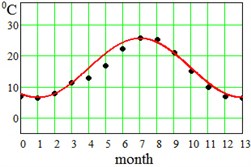
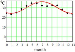
where approximation parameter – is the multi-year averaged mean temperature value, – is the amplitude of seasonal oscillations, and – is a delay. Said parameters have been found for each region and displayed at the bottom of the Table 1. This approximation by Eq. (5) is visualized in Fig. 2 for the error evaluation. From Fig. 2 it is seen that approximation by Eq. (5) works almost perfectly for regions Dallas, Hong-Kong and Shimkent regions, and slightly worse for Madrid, Delhi, Singapore and Khartoum.
2.2. Diurnal temperature model
Further, one could extract daily air temperature oscillations from monthly average maximum and average minimum data available from weather services [18-29], assuming that average maximums and minimums correspond to the day time maximum and night time minimum of temperatures oscillations.
Table 1Daily mean air temperature by months, °C
Data source | [18] | [20] | [22] | [23] | [25] | [27] | [28] |
Observation period | 1949-1989 | 1981-2010 | 2008-2017 | 1981-2010 | 1971-1990 | 1981-2010 | 1971-2000 |
Region | Dallas, USA | Hong-Kong, China | Chimkent, Kazakhstan | Madrid, Spain | Delhi, India | Singapore | Khartoum, Sudan |
Jan | 6,9 | 18,6 | –0,7 | 6,3 | 14,3 | 26,5 | 23,2 |
Feb | 9,4 | 18,8 | 1,6 | 7,9 | 16,8 | 27,1 | 25 |
Mar | 13,6 | 21,4 | 7,6 | 11,2 | 22,3 | 27,5 | 28,7 |
Apr | 18,6 | 25,0 | 13,6 | 12,9 | 28,8 | 28 | 31,9 |
May | 22,9 | 28,4 | 19,1 | 16,7 | 32,5 | 28,3 | 34,5 |
Jun | 27,0 | 30,2 | 23,7 | 22,2 | 33,4 | 28,3 | 34,3 |
Jul | 29,5 | 31,4 | 26,3 | 25,6 | 30,8 | 27,9 | 32,1 |
Aug | 29,3 | 31,1 | 25,3 | 25,1 | 30 | 27,9 | 31,5 |
Sep | 25,3 | 30,1 | 19,9 | 20,9 | 29,5 | 27,6 | 32,5 |
Oct | 19,7 | 27,8 | 12,3 | 15,1 | 26,3 | 27,6 | 32,4 |
Nov | 13,1 | 24,1 | 6,4 | 9,9 | 20,8 | 27 | 28,1 |
Dec | 8,6 | 20,2 | 0,9 | 6,9 | 15,7 | 26,4 | 24,5 |
Approximation parameters | |||||||
18,3 | 25,4 | 13,0 | 16,0 | 25,1 | 27,4 | 30,0 | |
11,5 | 6,5 | 13.8 | 9,5 | 9,0 | 1,0 | 6,0 | |
1.1 month | 1.4 months | 1 month | 1 month | 0.8 months | 0 months | 1 month | |
Fig. 2Average seasonal temperature approximations. Dotted lines-data from Table 1, continues lines – approximation by Eq. (5)
a) Dallas, USA
b) Hong-Kong, China
c) Shimkent, Kazakhstan
d) Madrid, Spain
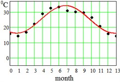
e) Delhi, India
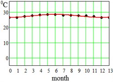
f) Singapore
g) Khartoum, Sudan
In Table 2 here are monthly average maximum and minimum data for the regions under consideration. On Fig. 3 here are illustrations of the averaged daily temperature swings due to the diurnal oscillation above and below daily mean values plotted for each month of an year. This swings have been obtained by subtracting average monthly mean values of Table 1 from average maximum and minimum values of Table 2. On Fig. 3 ± is the border within which the diurnal temperatures oscillate around the daily mean.
Fig. 3Average maximum and minimum temperatures. Black dots – data combined from Table 1 and Table 2, red lines – approximation amplitude Tda by Eq. (6)
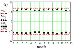
a) Dallas, USA
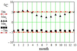
b) Hong-Kong, China
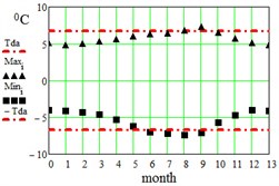
c) Shimkent, Kazakhstan
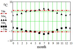
d) Madrid, Spain
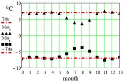
e) Delhi, India
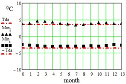
f) Singapore
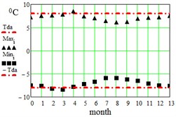
g) Khartoum, Sudan
In science literature [30-33] there are a variety of ways suggested to model shape of the diurnal temperature curves. Methods based on energy budget models require a large number of input parameters. Methods based on empirical models are sinusoidal models which only require maximum and minimum temperature and some parameters as input. Proposed sinusoidal models are combinations of periodic sine and exponential decay curves or linear decay curves, they are multi-parameter models and are not easily represented by a few terms. Except for pure sinusoidal model others require location latitude and longitude to calculate sunrise and sunset times to determine parametric phases of piecewise defined fitting curves. To better approximate empirical data model parameters should be dependent on year seasons, that would complicate calculation of a life time. For the first step evaluation purposes let us exploit a simple sine function with an empirical amplitude parameter , a fixed 24 hour period day, and some phase to model diurnal temperatures oscillations:
For model examination, on Fig. 4 here are graphs of the ambient temperature with zero fluctuation 0 and of monthly averaged maximums and minimums given for Shimkent region.
Fig. 4Approximation of seasonal and daily temperature oscillations, Shimkent region, To= +13.0 °С, Tsa= +13.8 °С, Tda= +6.7 °С, to= 1 month, ΔTt= 0
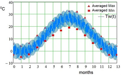
Table 2Daily average maximum and minimum air temperature by months, °C
Data source | [18] | [20] | [22] | [23] | [25] | [27] | [28] | |||||||
Observ. period | 1948-2003 | 1981-2010 | 2008-2017 | 1981-2010 | 1971-1990 | 1981-2010 | 1971-2000 | |||||||
Region | Dallas, USA | Hong-Kong, China | Chimkent, Kazakhstan | Madrid, Spain | Delhi, India | Singapore | Khartoum, Sudan | |||||||
Average | max | low | max | low | max | low | max | low | max | low | max | low | max | low |
Jan | 12,8 | 1 | 23,7 | 14,5 | 4,1 | –4,8 | 9,8 | 2,7 | 21 | 7,6 | 30,4 | 23,9 | 30,7 | 15,6 |
Feb | 15,6 | 3,3 | 24,5 | 15 | 6,6 | –2,7 | 12 | 3,7 | 23,5 | 10,1 | 31,7 | 24,3 | 32,6 | 16,8 |
Mar | 19,9 | 7,4 | 27,1 | 17,2 | 12,9 | 3 | 16,3 | 6,2 | 29,2 | 15,3 | 32 | 24,6 | 36,5 | 20,3 |
Apr | 24,7 | 12,5 | 29,8 | 20,8 | 19,2 | 8,3 | 18,2 | 7,7 | 36 | 21,6 | 32,3 | 25 | 40,4 | 24,1 |
May | 28,6 | 17,2 | 31,8 | 24,1 | 25,1 | 12,9 | 22,2 | 11,3 | 39,2 | 25,9 | 32,2 | 25,4 | 41,9 | 27,3 |
Jun | 32,8 | 21,3 | 33,1 | 26,2 | 30 | 16,7 | 28,2 | 16,1 | 38,8 | 27,8 | 32 | 25,4 | 41,3 | 27,6 |
Jul | 35,5 | 23,6 | 33,8 | 26,8 | 32,7 | 19,1 | 32,1 | 19 | 34,7 | 26,8 | 31,3 | 25 | 38,5 | 26,2 |
Aug | 35,5 | 23,2 | 33,8 | 26,6 | 32,1 | 17,9 | 31,3 | 18,8 | 33,6 | 26,3 | 31,4 | 25 | 37,6 | 25,6 |
Sep | 31,3 | 19,4 | 33,8 | 25,8 | 27,2 | 12,8 | 26,4 | 15,4 | 34,2 | 24,7 | 31,4 | 24,8 | 38,7 | 26,3 |
Oct | 26,1 | 13,3 | 30,8 | 23,7 | 18,8 | 6,6 | 19,4 | 10,7 | 33 | 19,6 | 31,7 | 24,7 | 39,3 | 25,9 |
Nov | 19,2 | 7,1 | 28 | 19,8 | 12,1 | 1,7 | 13,5 | 6,3 | 28,3 | 13,2 | 31,1 | 24,3 | 35,2 | 21 |
Dec | 14,4 | 2,8 | 25,1 | 15,9 | 6 | –3,1 | 10 | 3,6 | 22,9 | 8,5 | 30,2 | 24 | 31,7 | 17 |
Approximation values | ||||||||||||||
6,7 | 5,0 | 6,7 | 5,5 | 7,0 | 3,5 | 8,0 | ||||||||
2.3. Temperature fluctuations
Because we believe that modeled and curves are very close to true average values, in Eq. (4) is considered to account only for random temperature deviations from average. Therefore, in that assumption the mean expectation value is zero. Temperature fluctuations of any nature although with zero mean value will bias the life time estimation because of non-linearity of Eq. (2). Thus, the influence of random fluctuations should be considered. There are some data, for example, record high and record low temperature values provided by weather services [18-29] that could be usefully applied. Record high excess over average high is a maximum positive fluctuation, record low drop below average minimum is a maximum negative fluctuation. On Fig. 5 there are plotted maximum positive and negative fluctuation values in months given for regions under consideration. Positive maximum fluctuations have been found by subtracting average daily maximum from record high provided by [18-29], negative maximum fluctuations have been found by subtracting average daily minimum from record minimum provided by [18-29].
From presented Fig. 4 it will not be a big error if the fluctuation range will be considered constant over time for simplicity. Other simplification is that the standard deviation is assumed to be constant over time.
Fig. 5Record high Rmax and record low Rlow temperature fluctuations. Black dots - data combined from statistical data, red lines – approximation swing amplitude ΔTa. Regions: a) Dallas, USA, ΔTa= 14 °C, observing period 1948-2017 data source – [19]; b) Hong-Kong, China, ΔTa= 4 °C, observing period 1947-2018 data source – [21]; c) Shimkent, Kazakhstan, ΔTa= 16 °C, observing period 2008-2017 data source – [22]; d) Madrid, Spain, ΔTa= 11 °C, observing period 1981-2010 data source – [24]; e) Delhi, India, ΔTa= 9 °C, observing period 1971-2010 data source – [26]; f) Singapore, ΔTa= 5 °C, observing period 1920-2017 data source – [27]; g) Khartoum, Sudan, ΔTa= 9 °C, observing period 1961-1990 data source – [29]
![Record high Rmax and record low Rlow temperature fluctuations. Black dots - data combined from statistical data, red lines – approximation swing amplitude ΔTa. Regions: a) Dallas, USA, ΔTa= 14 °C, observing period 1948-2017 data source – [19]; b) Hong-Kong, China, ΔTa= 4 °C, observing period 1947-2018 data source – [21]; c) Shimkent, Kazakhstan, ΔTa= 16 °C, observing period 2008-2017 data source – [22]; d) Madrid, Spain, ΔTa= 11 °C, observing period 1981-2010 data source – [24]; e) Delhi, India, ΔTa= 9 °C, observing period 1971-2010 data source – [26]; f) Singapore, ΔTa= 5 °C, observing period 1920-2017 data source – [27]; g) Khartoum, Sudan, ΔTa= 9 °C, observing period 1961-1990 data source – [29]](https://static-01.extrica.com/articles/20733/20733-img17.jpg)
a)
![Record high Rmax and record low Rlow temperature fluctuations. Black dots - data combined from statistical data, red lines – approximation swing amplitude ΔTa. Regions: a) Dallas, USA, ΔTa= 14 °C, observing period 1948-2017 data source – [19]; b) Hong-Kong, China, ΔTa= 4 °C, observing period 1947-2018 data source – [21]; c) Shimkent, Kazakhstan, ΔTa= 16 °C, observing period 2008-2017 data source – [22]; d) Madrid, Spain, ΔTa= 11 °C, observing period 1981-2010 data source – [24]; e) Delhi, India, ΔTa= 9 °C, observing period 1971-2010 data source – [26]; f) Singapore, ΔTa= 5 °C, observing period 1920-2017 data source – [27]; g) Khartoum, Sudan, ΔTa= 9 °C, observing period 1961-1990 data source – [29]](https://static-01.extrica.com/articles/20733/20733-img18.jpg)
b)
![Record high Rmax and record low Rlow temperature fluctuations. Black dots - data combined from statistical data, red lines – approximation swing amplitude ΔTa. Regions: a) Dallas, USA, ΔTa= 14 °C, observing period 1948-2017 data source – [19]; b) Hong-Kong, China, ΔTa= 4 °C, observing period 1947-2018 data source – [21]; c) Shimkent, Kazakhstan, ΔTa= 16 °C, observing period 2008-2017 data source – [22]; d) Madrid, Spain, ΔTa= 11 °C, observing period 1981-2010 data source – [24]; e) Delhi, India, ΔTa= 9 °C, observing period 1971-2010 data source – [26]; f) Singapore, ΔTa= 5 °C, observing period 1920-2017 data source – [27]; g) Khartoum, Sudan, ΔTa= 9 °C, observing period 1961-1990 data source – [29]](https://static-01.extrica.com/articles/20733/20733-img19.jpg)
c)
![Record high Rmax and record low Rlow temperature fluctuations. Black dots - data combined from statistical data, red lines – approximation swing amplitude ΔTa. Regions: a) Dallas, USA, ΔTa= 14 °C, observing period 1948-2017 data source – [19]; b) Hong-Kong, China, ΔTa= 4 °C, observing period 1947-2018 data source – [21]; c) Shimkent, Kazakhstan, ΔTa= 16 °C, observing period 2008-2017 data source – [22]; d) Madrid, Spain, ΔTa= 11 °C, observing period 1981-2010 data source – [24]; e) Delhi, India, ΔTa= 9 °C, observing period 1971-2010 data source – [26]; f) Singapore, ΔTa= 5 °C, observing period 1920-2017 data source – [27]; g) Khartoum, Sudan, ΔTa= 9 °C, observing period 1961-1990 data source – [29]](https://static-01.extrica.com/articles/20733/20733-img20.jpg)
d)
![Record high Rmax and record low Rlow temperature fluctuations. Black dots - data combined from statistical data, red lines – approximation swing amplitude ΔTa. Regions: a) Dallas, USA, ΔTa= 14 °C, observing period 1948-2017 data source – [19]; b) Hong-Kong, China, ΔTa= 4 °C, observing period 1947-2018 data source – [21]; c) Shimkent, Kazakhstan, ΔTa= 16 °C, observing period 2008-2017 data source – [22]; d) Madrid, Spain, ΔTa= 11 °C, observing period 1981-2010 data source – [24]; e) Delhi, India, ΔTa= 9 °C, observing period 1971-2010 data source – [26]; f) Singapore, ΔTa= 5 °C, observing period 1920-2017 data source – [27]; g) Khartoum, Sudan, ΔTa= 9 °C, observing period 1961-1990 data source – [29]](https://static-01.extrica.com/articles/20733/20733-img21.jpg)
e)
![Record high Rmax and record low Rlow temperature fluctuations. Black dots - data combined from statistical data, red lines – approximation swing amplitude ΔTa. Regions: a) Dallas, USA, ΔTa= 14 °C, observing period 1948-2017 data source – [19]; b) Hong-Kong, China, ΔTa= 4 °C, observing period 1947-2018 data source – [21]; c) Shimkent, Kazakhstan, ΔTa= 16 °C, observing period 2008-2017 data source – [22]; d) Madrid, Spain, ΔTa= 11 °C, observing period 1981-2010 data source – [24]; e) Delhi, India, ΔTa= 9 °C, observing period 1971-2010 data source – [26]; f) Singapore, ΔTa= 5 °C, observing period 1920-2017 data source – [27]; g) Khartoum, Sudan, ΔTa= 9 °C, observing period 1961-1990 data source – [29]](https://static-01.extrica.com/articles/20733/20733-img22.jpg)
f)
![Record high Rmax and record low Rlow temperature fluctuations. Black dots - data combined from statistical data, red lines – approximation swing amplitude ΔTa. Regions: a) Dallas, USA, ΔTa= 14 °C, observing period 1948-2017 data source – [19]; b) Hong-Kong, China, ΔTa= 4 °C, observing period 1947-2018 data source – [21]; c) Shimkent, Kazakhstan, ΔTa= 16 °C, observing period 2008-2017 data source – [22]; d) Madrid, Spain, ΔTa= 11 °C, observing period 1981-2010 data source – [24]; e) Delhi, India, ΔTa= 9 °C, observing period 1971-2010 data source – [26]; f) Singapore, ΔTa= 5 °C, observing period 1920-2017 data source – [27]; g) Khartoum, Sudan, ΔTa= 9 °C, observing period 1961-1990 data source – [29]](https://static-01.extrica.com/articles/20733/20733-img23.jpg)
g)
3. Influence of air temperature fluctuations on a capacitor life time
To improve reliability for outdoor applications, electronic devices are usually sealed to prevent from moisture, dust, insects and other foreign objects. Therefore, for the components inside a device enclosure the difference in ambient temperature is the only significant difference between outdoor and indoor operation. The steady-state temperature inside the case of an operating device linearly depends on the external temperature in the first approximation. Let (25 °С) be the temperature inside the case measured at the ambient air temperature +25 °С, then it is possible to predict with confidence the temperature inside the case under other ambient temperature : () = (25 °С) + ( – 25 °С). One could rewrite Eq. (1) in the form:
where – time to failure under certain constant operating conditions and the temperature inside the device enclosure referenced to ambient room temperature 25 °C. Suppose that an operating device has a temperature 84 °C inside the case, then is the operating time in these stationary conditions that cloud be found earlier with standard calculations or measurements in a laboratory. If the device does not work, then inside the case 25 °C, and is the storage time at the 25 °C room temperature or in other words in a laboratory conditions. is obviously with different , applied voltage and so on. Let us assume, that the device operates all the time throughout years having regular day by day diurnal scheduler. In derivations below it is supposed that the device is not exposed to the direct sun irradiation. Substituting Eq. (4) for and Eq. (7) for into Eq. (2), one can get:
where – is the average temperature which obviously has the one year repetitive period. For a moment, let us suppose that the end result is equal to the integer number of years , then one could further rewrite Eq. (8):
where now have got a peace-wise representation as a number of functions , each of which is valid for a given year . Notice that and are not indexed with because they are independent of the a specific year, therefore one could put sum by years inside the year integral:
If the number of expected working years is big enough, for example 10 years or more, then one could rewrite Eq. (10) in terms of the mean expected value for :
And the longer the life time ( ∞) the more precise Eq. (11) will be. In our model for the outdoor air temperature it was assumed that has a constant probability distribution therefore is constant. Therefore, one could get:
The diurnal temperature changes by time much faster than the seasonal temperature , actually 365 times faster, thus one can consider constant during diurnal time period. The values of slowly varying seasonal oscillations were taken as constants on the diurnal intervals of an integration and therefore seasonal dependencies as multipliers were taken out of the daily integral signs. And the entire continuous integral is replaced by the sum (over days) of piecewise daily integrals with the corresponding seasonal weights for each day, having obtained for the right side of the Eq. (12):
Notice that and are not indexed with because they are independent of a specific day, therefore one could take the daily integral out of sum brackets, and the sum itself was replaced with an year integral:
Let us rewrite Eq. (12) one more time in a way suitable for visual perception taking into account Eq. (14) and that , then:
where and are downgrading coefficients associated with temperature fluctuations and multi-year averaged seasonal temperatures oscillations:
If the temperature fluctuation was modeled with an equal probability distribution over the deviation range [], one could get numerical evaluation for the fluctuation contribution on a capacitor life time:
If in Eq. (17) one uses Eq. (5) for then one could find that splits into two multipliers such as:
is the coefficient associated with the fact that the capacitor is subject to weather conditions where the average annual temperature differs from room temperature 25 °C. is the decreasing coefficient associated with seasonal oscillations of multi-year averaged temperatures, that can be expressed through modified Bessel function Io of the first kind. The coefficients , , have been calculated for regions under consideration and listed on Table 3 to judge contributions of the temperature components.
The mean multi-year air temperature has a much greater impact on a capacitor life time since the multi-year mean could differ from the room temperature by more than 10 °C. The regions closer to the equator Khartoum, Singapore, and Hong-Kong are warmer, therefore decreasing coefficients are bigger, with the highest value 1.41 for the hottest Khartoum from listed regions. Seasonal coefficients are bigger for inland regions with a continental climate, like located far from equator Chimkent, Dallas and Madrid, therefore having increased seasonal air temperature oscillations although lowered annual means. Chimkent has a sharply continental climate with highest among the regions resulting 1.24. As a rule, for regions with a continental climate it is worth to estimate decreasing coefficient . For example, for Chimkent and Dallas these coefficients would have significant 22 % and 17 % contributions correspondingly. Coefficient is quiet miserable for mild climates such as Hong-Kong and Singapore. In Table 3 the is the total decreasing coefficient ***.
Table 3Correction coefficients
Region | ||||||
Dallas, USA | 0.629 | 1.165 | 1.055 | 1.165 | 1,23 | 0.90 |
Hong-Kong, China | 1.028 | 1.051 | 1.03 | 1.013 | 1,04 | 1.13 |
Chimkent, Kazakhstan | 0.435 | 1.242 | 1.055 | 1.218 | 1,28 | 0.70 |
Madrid, Spain | 0.536 | 1.111 | 1.037 | 1.100 | 1,14 | 0.68 |
Delhi, India | 1.007 | 1.100 | 1.060 | 1.066 | 1,13 | 1.25 |
Singapore | 1.181 | 1.001 | 1.015 | 1.020 | 1,04 | 1.22 |
Khartoum, Sudan | 1.414 | 1.044 | 1.078 | 1.066 | 1,15 | 1.70 |
4. Constant load
Let us suppose that a device operates around the clock under constant load, therefore is a constant during diurnal integral and Eq. (15) can be further expanded:
where:
is the decreasing coefficient associated with daily oscillations of multi-year averaged temperatures. The has been calculated for regions under consideration and listed on Table 3 for the contribution estimation. From which it is noticeable, the influence of averaged daily oscillations on an electrolytic capacitor life time evaluation are quiet moderate. And once again for regions like Dallas, Madrid, Shimkent, Delhi, and Khartoum with a continental climate the coefficients accounting daily temperature oscillations are higher with the highest 8 % contribution for Khartoum, although the Khartoum seasonal average temperature amplitude do not exceeds 6 °C due to proximity to the equator. Coefficient is quiet low for localities with mild climate like Hong-Kong and Singapore.
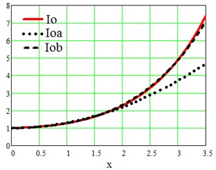
On Fig. 6 one can see illustration of Bessel function dependence on its argument.
The Bessel function is rather rapidly converging sum of power series of its argument. Some simple approximation functions might be helpful. The quadratic function:
approximates quite well the Bessel function Io in the range of –26 °С to 26 °С, that is enough to successfully evaluate Io for temperature fluctuations on the earth's surface. And the function:
works quite well, see Fig. 6, for an extended range of temperature oscillations –48 °C to 48 °C.
During operation a capacitor may undergo alternating RMS currents or alternating voltages, and if this oscillations are much faster than diurnal period then in Eq. (21) might include effect-integrating values of those parameters.
The original Eq. (8) does not decompose into a coefficient product , but calculations with help of Eq. (21) give values close to numerically calculated by Eq. (8) with great accuracy.
Fig. 6Iox – Bessel function. Ioax and Iobx – approximations of Bessel function Io
5. Variable load
The derivation of Eq. (21) was carried out for a device operating around the clock. However, not all devices work in this mode. For example, street lighting devices work at night, telecommunication devices are actively loaded at a daytime. In Eq. (15) the is not constant under variable load, due to voltage , current and other operating parameters change. Let us consider a hypothetical device, for example, LED lamp operating only at nights and calculate its hypothetical capacitor service life in comparison with the life time at room temperature and continues around-the-clock operation. Let us assume that the device operates 12 hours from 20.00 hour in the evening until 8.00 hour at the morning. During the daytime the imaginary LED lamp is turned off, the temperature inside the LED power supply case is set equal to the outdoor air temperature, if no additional heating measures are provided. For convenience let us rewrite Eq. (15) one more time in a way suitable for visual perception:
where is the day interval where the device operates, and is the day interval where it is turned off, while 24 hour is ever true. If one use the simple model Eq. (6) for to substitute it in Eq. (25) then:
where is ever true. In order to calculate the coefficients at and , for certain let us assume that the LED lamp operates at the moments of the lowest temperatures, that is, at the cosine positive half-wave, when –0.5, 0.5 and 1.5. And, to be specific, for a particular locality like Shimkent with highest daily average temperature maximums and minimums it could be found:
Thus, in Eq. (27), for a time to failure of a hypothetical street lamp operating in Shimkent region one have got a correction factor 0.376 for night cold time of a day and a coefficient 0.679 for a warm daytime. The sum of day and night coefficients 0.376 + 0.679 from Eq. (27) is equal to the reduction coefficient for Shimkent from Table 3. Since the device operates at night, the coefficient 0.376 is at , and the day coefficient 0.679 is at . From Eq. (27) it is clearly seen that it does matter which part of the day the device works, because day and night coefficients significantly differ by factor of about two for the particular locality with continental climate and given temperature model . The formula of Eq. (25) is quiet sensitive to the implemented model shape of the diurnal temperature curves. Therefore, for better evaluation more accurate but a bit complicated diurnal models [30-33] exploiting combination of periodic sine for daytime and exponential decay curves or linear decay curves for night time must be recommended.
6. Conclusions
The Miner's principle is frequently used to evaluate electrolytic capacitor life time under variable thermal stresses. In the work easy-to-use analytical approach was proposed to avoid bulky numerical calculations. Outdoor air temperature change was modeled by sum of four components – the average multi-year temperature, the averaged multi-year seasonal changes, the averaged daily temperature changes and temperature fluctuations. With this model the Miner’s formula for the electrolytic capacitor life time estimation was modified in a way that the contribution of each individual temperature phenomenon can be evaluated. Therefore the purpose of the work, to get handy evaluation tool of daily temperature oscillation and temperature fluctuation contributions, have been reached. Moreover, it is possible to introduce a reference table with pre-calculated constant correction coefficients for climatic regions of interest to estimate the electrolytic capacitor life time compared to a standard laboratory operating condition.
The correction coefficients corresponding to average daily temperature oscillations have a moderate contributions into a capacitor life time. The temperature fluctuations can have a greater impact on a life time estimation formula. From Table 3 it is seen that for some regions of a continental climate type (Dallas, Shimkent) the combined effect of average daily temperature oscillation and temperature fluctuations can reach sufficient correction values up to 30 %, therefore it is worth of estimation. If a device operates fraction of a day, the device's daily scheduler have significant impact on a resulting capacitor service time, and the calculations are quiet sensitive to the applied average daily temperature curve model.
The resulting formulas will be useful for engineering calculations of reliability in the development of electrical devices for outdoor applications but not exposed to direct sun irradiation. The obtained results can be used in further real-time outdoor experiments to confirm Miner's principle applicability.
References
-
Lahyani A., Venet P., Grellet G., Viverge P. Failure prediction of electrolytic capacitors during operation of a switchmode power supply. IEEE Transactions on Power Electronics, Vol. 13, 1998, p. 1199-1207.
-
Vorperian V. Simplified analysis of PWM converters using model of PWM switch continuous conduction mode. IEEE Transactions on Aerospace and Electronic Systems, Vol. 26, Issue 3, 1990, p. 490-496.
-
Sun B., Fan X., Qian C., Zhang G. PoF-simulation-assisted reliability prediction for electrolytic capacitor in LED drivers. IEEE Transactions on Industrial Electronics, Vol. 63, Issue 11, 2016, p. 6726-6735.
-
Wang H., Blaabjerg F. Reliability of capacitors for DC-link applications in power electronic converters – an overview. IEEE Transactions on Industry Applications, Vol. 50, Issue 5, 2014, p. 3569-3578.
-
Naikan V. N. A., Rathore A. Accelerated temperature and voltage life tests on aluminium electrolytic capacitors: A DOE approach. The International Journal of Quality and Reliability Management, Vol. 33, Issue 1, 2016, p. 120-139.
-
Kulkarni C. S., Celaya J. R., Biswas G., Goebel K. Accelerated aging experiments for capacitor health monitoring and prognostics. IEEE AutoTestCon, Anaheim, CA, 2012.
-
Whitman C. S. Impact of ambient temperature set point deviation on Arrhenius estimates. Microelectronics Reliability, Vol. 52, 2012, p. 2-8.
-
Bhargava Cherry, Banga Vijay Kumar, Singh Yaduvir An intelligent prognostic model for electrolytic capacitors health monitoring: a design of experiments approach. Advances in Mechanical Engineering, Vol. 10, Issue 10, 2018, https://doi.org/10.1177/1687814018781170.
-
Gupta Anunay, Yadav Om Prakash, Devoto Douglas, Major Joshua A review of degradation behavior and modeling of capacitors: preprint. International Technical Conference and Exhibition on Packaging and Integration of Electronic and Photonic Microsystems, 2018.
-
Miner M. Cumulative damage in fatigue. Journal of Applied Mechanics, Vol. 12, 159, p. 164-1945.
-
Albertini A., Masi M. G., Mazzanti G., Peretto L., Tinarelli R. Toward a BITE for real-time life estimation of capacitors subjected to thermal stress. IEEE Transactions on Instrumentation and Measurement, Vol. 60, Issue 5, 2011, p. 1674-1681.
-
Toshihiko Furukawa, Daizou Senzai, Takahiro Yoshida Electrolytic capacitor thermal model and life study for forklift motor drive application. World Electric Vehicle Symposium and Exhibition (EVS27), 2013.
-
Technical Notes for Electrolytic Capacitor. Rubycon Corporation, http://www.rubycon.co.jp/en/products/alumi/pdf/life.pdf.
-
Technical Note: Aluminum Electrolytic Capacitors. Elna corporation, http://www.elna.co.jp/en/capacitor/alumi/catalog/pdf/al_tecnote_e.pdf.
-
Nippon Chemi-con Corporation. Technical Note: Aluminum electrolytic capacitors. Lifetime of Aluminum Electrolytic Capacitors, p. 392-394, http://www.chemi-con.co.jp/e/catalog/pdf/al-e/al-all-e1001s-2018.pdf.
-
Albertsen A. Electrolytic Capacitor Lifetime Estimation. Jianhai Europe Electronic Components GmbH, 2012.
-
Historical weather observations and statistics. Australian Bureau of Meteorology (BOM), http://www.bom.gov.au/climate/data-services/station-data.shtml.
-
Station Name: TX DALLAS LOVE FLD. National Oceanic and Atmospheric Administration, 2013. ftp://ftp.ncdc.noaa.gov/pub/data/normals/1981-010/products/station/USW00013960.normals.txt.
-
NOWData – NOAA Online Weather Data. National Oceanic and Atmospheric Administration, https://www.nws.noaa.gov/climate/ xmacis.php?wfo=fwd.
-
Monthly Meteorological Normals for Hong Kong. Hong Kong Observatory, http://www.weather.gov.hk/cis/normal/1981_2010/normals_e.htm/.
-
Extreme Values and Dates of Occurrence of Extremes of Meteorological Elements between 1884-1939 and 1947-2017 for Hong Kong. Hong Kong Observatory, http://www.hko.gov.hk/cis/extreme /mon_extreme_e.htm.
-
Weather and Climate – The Climate of Shymkent. Weather and Climate, http://www.pogodaiklimat.ru/climate/38328.htm.
-
Valores climatológicos normales. Madrid, Retiro. AEMet, http://www.aemet.es/es/serviciosclimaticos /datosclimatologicos/valoresclimatologicos?l=3195&k=mad.
-
Extreme Values, Madrid. AEMet, http://www.aemet.es/en/serviciosclimaticos/datosclimatologicos /efemerides_extremos.
-
New Delhi (SFD) 1971-1990. National Oceanic and Atmospheric Administration, ftp://ftp.atdd.noaa.gov/pub/GCOS/WMO-Normals/RA-II/IN/42182.TXT.
-
Ever Recorded Maximum and Minimum Temperatures up to 2010. Indian Meteorological Department, http://www.imdpune.gov.in/ Temp_Extremes/histext2010.pdf.
-
Weather Statistics. National Environment Agency, Singapore, https://www.nea.gov.sg/weather-climate/climate/weather-statistics.
-
World Weather Information Service – Khartoum. World Meteorological Organization, http://worldweather.wmo.int/en/city.html?cityId=249.
-
Khartoum Climate Normals 1961–1990. National Oceanic and Atmospheric Administration, ftp://ftp.atdd.noaa.gov/pub/GCOS/WMO-Normals/TABLES/REG__I/SU/62721.TXT.
-
Reicosky D. C., Winkelman L. J., Baker J. M., Baker D. G. Accuracy of hourly air temperatures calculated from daily minima and maxima. Agricultural and forest Meteorology, Vol. 46, 1989, p. 193-209.
-
Deshani K. A. D., Liwan Liyanage Hansen Incorporating influential factors in diurnal temperature estimation with sparse data. GSTF Journal of Mathematics, Statistics and Operations Research (JMSOR), Vol. 3, Issue 2, 2016, p. 12-16.
-
Baker J. M., Reicosky D. C., Baker D. G. Estimating the time dependence of air temperature using daily maxima and minima: a comparison of three methods. Journal of Atmospheric and Oceanic Technology, Vol. 5, 1988, p. 736-742.
-
Eccel Emanuele What we can ask to hourly temperature recording. Part II: hourly interpolation of temperatures for climatology and modelling. Italian Journal of Agrometeorology, Vol. 2, 2010, p. 45-50.
About this article

The work was funded by the Science Committee of the Ministry of Education and Science of the Republic of Kazakhstan in the framework of the project AP No. 05135334 “Research and Development of an Innovative Micro-Inverter for Photovoltaic Panels”.
