Abstract
In order to research the influence of the control delay time on the vibration isolation system, the dynamic characteristic analysis of a two-degree-of-freedom vibration system, based on high-static-low-dynamic-stiffness vibration isolator (HSLDS-VI) with time-delayed feedback control is presented. The two-degree-of-freedom nonlinear vibration isolation dynamical system model comprising the delay time parameter is also derived. Then, the effects of feedback gain coefficient and delay parameter on the dynamic characteristics are analyzed with multiple scales method. The results demonstrate that the amplitude can be suppressed by the time-delay variation for a fixed feedback gain. The system can exhibit periodic motion or chaotic vibration when the feedback gain coefficient and time-delay parameter are adjusted, which is beneficial to the application of high-static-low-dynamic-stiffness vibration isolator.
Highlights
- In order to research the influence of the control delay time, the mathematical model of the two-degree-of-freedom nonlinear vibration system based on the HSLDS-VI is established
- The influence of time-delayed feedback on the system vibration amplitude is investigated by multiple scales method, and the system has different responses with the increase of the time delay
- The analytical solution is in good agreement with the numerical results, the system exhibit periodic or chaotic vibration with the parameters, which is beneficial to the application of the HSLDS-VI
1. Introduction
How to suppress low-frequency vibration effectively has always been a concerned issue in the field of vibration control. In general, to increase the vibration isolation range, the system stiffness should be reduced at the same time, but this will reduce its loading capacity. To overcome this contraction, many scholars have proposed an isolator with high-static-low-dynamic-stiffness. The high-static-low-dynamic-stiffness vibration isolator (HSLDS-VI) is comprised of a positive and a negative stiffness structure. The former part is used to carry the main load, and the latter part is used to offset the stiffness of the positive mechanism, so that the system stiffness could equal to zero at the equilibrium position. Kovacic and Carrella et al. [1, 2] designed an HSLDS-VI by connecting two oblique springs as negative stiffness, and its amplitude-frequency and transmission characteristics were further studied in detail. Xu and Zhou et al. [3, 4] designed an HSLDS-VI by using the electromagnetic negative stiffness spring and conducted the theoretical and experimental analysis. Meng et al. [5] put forward to design HSLDS-VI with equal thickness and variable thickness butterfly spring, and the parameters influence on the transmission rate was studied as well. Huang [6] used the Euler buckling beam with negative stiffness to analyze the static and dynamic characteristics, the experimental results showed that the HSLDS-VI had a wider vibration isolation band than the linear isolator.
Meanwhile, the time-delay parameter has a direct influence on mechanical vibration feedback control. Hu et al. [7] studied the primary resonance and 1/3 harmonic resonance of the Duffing system with delayed state feedback method and applied at multiple scales methods to study the required gain and delay parameter values for effective vibration control. Olgac [8] proposed a time-delay resonator in a coupled linear forced vibration system to eliminate the vibration and obtained the theoretical basis and experimental results in time-delay vibration reduction. Maccari [9] studied the delayed feedback control method for suppressing large-valued response and quasi-periodic motion in Van der Pol oscillators and implemented this method to the control of the main resonance of a cantilever beam. Besides, Hosek [10] used a centrifugal pendulum time-delay resonator to control the torsional system, the vibration was removed by adjusting the feedback gain and time-delay online. Chatterjee [11] studied the acceleration delay feedback control method in a nonlinear mechanical vibration system. It was found that the delay acceleration feedback also affected the system's damping characteristics. Cheng [12] studied the HSLDS-VI dynamic analysis with the time-delayed feedback, results showed the appropriate feedback parameters could improve the vibration isolation performance.
At present, the influence of the controlling delay time on two-degree-of-freedom system with a high-static-low-dynamic-stiffness isolator is expected to be studied in detail. This paper establishes a mathematical model of multi-degree-of-freedom high-static-low-dynamic stiffness vibration system with time-delayed feedback control, and the dynamic characteristics are also researched under different delays and feedback gain parameters.
2. Static analysis of HSLDS-VI
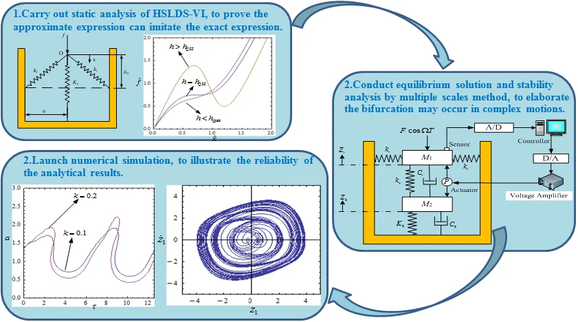
The HSLDS-VI schematic is shown in Fig. 1. Two oblique springs as negative stiffness and a vertical spring as positive stiffness are connected at point . The positive and negative stiffness are respectively, and the parameters and are defined as the system geometry, the coordinate x defines the displacement from the position .
Fig. 1the HSLDS-VI schematic
The expression between force and displacement is given by:
Introducing the non-dimensional parameters:
Eq. (1) can be rewritten as:
Differentiating Eq. (2), the non-dimensional stiffness can be given:
Let and , the conditions with the system zero stiffness can be obtained:
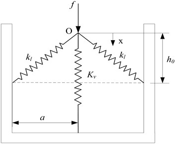
The non-dimensional force and stiffness for three conditions when the parameter are shown in Fig. 2. It can be seen that the system stiffness at the static equilibrium position is zero when the parameter , but the stiffness is always positive in the other range. If the parameter , the system will exhibit positive-stiffness continuously. Otherwise, if the parameter , the system stiffness will be negative at the static equilibrium position.
Fig. 2Non-dimensional force-displacement and stiffness-displacement curves of the HSLDS-VI (α=1)
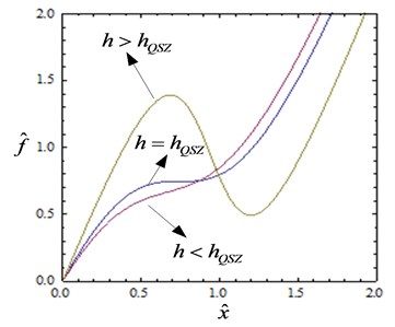
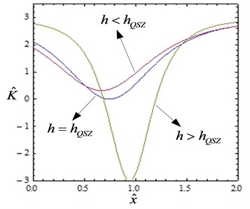
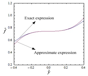
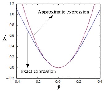
Fig. 3Comparison between the approximate and exact expressions of non-dimensional force and stiffness (α=1, h=hQZS)
When the displacement is small, Eq. (2) can be expanded by using a Taylor series at the static equilibrium position and let , we can get:
where, , . The non-dimensional stiffness can be obtained by differentiating Eq. (6):
The comparison between approximate and exact expressions of non-dimensional force and stiffness is illustrated in Fig. 3. The error between the two curves increases with the increase of displacement. When the amplitude of displacement at the static equilibrium position is small, the error can be taken into account. So the approximate expression can be used to imitate the exact expression.
3. Analysis by multiple scales method
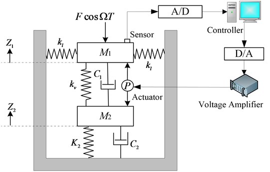
The two-degree-of-freedom system with time-delayed feedback is illustrated in Fig. 4. It includes an HSLDS-VI between the upper mass and middle mass , the linear stiffness spring between the middle mass and foundation. where, and are the vibration displacement, and are the system damping, the excitation force amplitude is , and its excitation frequency is . In addition, the actuator is installed between the upper and middle mass, so the control force can be expressed as .
Fig. 4Two-degree-of-freedom nonlinear vibration system with time-delayed feedback control
Thus, the system equations can be obtained according to Newton’s law of motion:
Substitute Eq. (5) into Eq. (7), and introduce the non-dimensional parameters:
The system non-dimensional equation can be get:
To analyze the main resonance by the multiple scales method, it is assumed that:
Where, . The forms of two-scale approximate expansion in Eq. (9) are assumed as:
Where, , . Using the following differential equations:
where, , ( 0, 1). Substituting Eqs. (9)-(14) into Eq. (8), and equating the coefficients of same power . If the power is zero, we can get:
If the power is one, we also can get:
The general solution of Eq. (15) and Eq. (16) can be set as:
where, and are undetermined functions, denotes the complex conjugate term. . The external excitation and time delay can be expressed as the following complex form:
Assuming and are very small, and can be expanded by using Taylor series:
Substitute Eqs. (19)-(24) into Eq. (17) and Eq. (18), we can obtain:
Considering the dynamic behavior when the primary resonance and the 1:1 internal resonance occur simultaneously. The deviation values are represented by the introduction of harmonic parameters and . The and denotes the external and internal resonance deviation value respectively:
The solvability conditions for Eq. (23) and (24) can be obtained:
The general solution of Eq. (29) and Eq. (30) can be written as the followings:
Substituting Eq. (31)-(32) into Eq. (29) and Eq. (30), and separating the real part from the imaginary part. We can obtain:
where, , .
4. Equilibrium solution and stability analysis
The system steady-state motion corresponds to the equilibrium solution of the equation . To further analyze the stability of the equilibrium solution, a perturbation analysis is performed on the Eqs. (33)-(36). The characteristic equation for the equilibrium solution can be obtained:
where, represents the eigenvalues of the Jacobian matrix, , , and are the coefficient of the characteristic equation. Using Roth-Hurwitz criterion to judge the stability of the equation, and the necessary and sufficient conditions of the system stability are obtained:
A sufficient and necessary condition for the stability of the equilibrium solution in Eq. (8) is the case that the real parts of all the characteristic roots in Eq. (35) are negative. If one of them is positive, then the equilibrium solution of Eq. (8) is not stable. If the real part of the characteristic root changes from the negative to the positive number, the system may have to saddle node bifurcation, which will lead to the emergence of jumping phenomenon. In addition, if the real part of a pair of complex eigenvalues changes from the negative to the positive number, Hopf bifurcation may occur in the system, which will result in complex periodic motions.
5. Simulation analysis
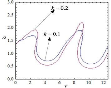
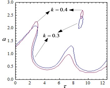
When the parameters , , , , , , , the amplitude with time-delayed curves are shown in Fig. 5. When the feedback gain is constant, the system vibration amplitude fluctuates with the time delay. It can be observed that the vibration amplitude can be reduced by adjusting the delay time. When the feedback gain coefficient is small, the system steady-state solution is a stable solution. Even if the system takes a large delay, the system remains stable at the equilibrium solution. When the feedback gain increases to 0.2, the system will have unstable solutions in some areas as the delay changes. This means that complex motions such as quasi-periodic motion and chaotic motion will appear in some regions. At the same time, it can be seen from Fig. 6(a) that the system vibration amplitude decreases as the feedback gain increases when [3, 8]. As the feedback gain is further increased, the system will have multiple stable solutions when some delay values are taken (for example ). This implies that the system will exhibit complex movements.
Fig. 5Amplitude and time-delayed curves with different feedback gains
a)
b)
Fig. 6Time response curves with several values of feedback gain and delay
a),
b),
c),
d),
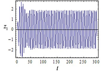
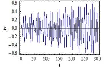
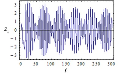
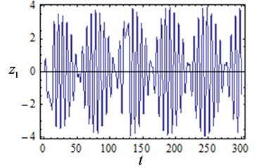
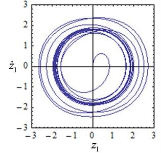
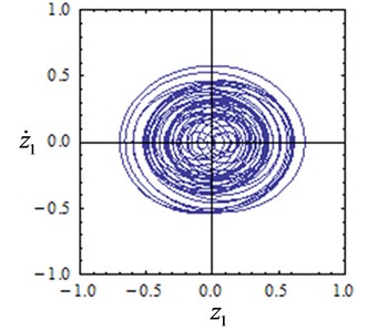
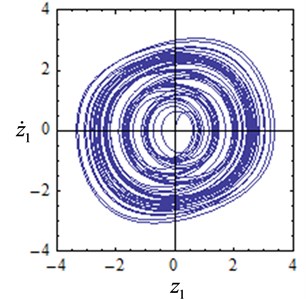
To illustrate the reliability of the above results, numerical verification of the results in Fig. 5 is conducted. The system time response curves are shown in Fig. 6, and the phase diagrams are shown in Fig. 7. The initial condition is set as 0.0001, 0.0001. The response characteristic curves are shown in Fig. 6(a) and Fig.7(a) when the feedback gain is 0.1 and the delay is 3, and the system exhibits a stable periodic motion. It can be seen from Fig. 6(b) and Fig. 7(b) that the system is chaotic at this time when the feedback gain is 0.2 and the delay is 2.7. As is shown in Figs. 6(c)-(d) and Figs. 7(c)-(d) when the feedback gain is 0.3, 0.4 and the delay is 9, the system shows multiple periodic motions. The numerical results are compared with Fig. 5 and it is found that the numerical simulation results are consistent with the analytical results, which indicates that the conclusions obtained in this paper are reliable.
Fig. 7Phase diagrams with several values of feedback gain and delay
a),
b),
c),
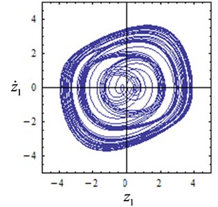
d),
6. Conclusions
In this paper, the mathematical model of the two-degree-of-freedom nonlinear vibration system based on a high-static-low-dynamic-stiffness isolator with time-delayed feedback is established. When the equations contain a delay term, the system exhibits more complex dynamic characteristics due to the influence of non-linear factors. The influence of time-delayed feedback on the system vibration amplitude is investigated by using multiple scales method, and the amplitude and time-delayed curves are also obtained for the two-degrees-of- freedom vibration system. It is observed that with the increase in time delay, the system has different responses. Through numerical analysis, it is found that the analytical solution is in good agreement with the numerical results. When the feedback gain coefficient is small, the system will be in a stable periodic motion. For a fixed feedback gain coefficient, the system vibration can be controlled by adjusting the time delay. With the increase of the feedback gain coefficient, the system will exhibit complex multiple-periodic and chaotic motion in certain time-delay regions.
References
-
Kovacic I., Brennan M. J., Lineton B. Effect of a static force on the dynamic behavior of a harmonically excited quasi-zero stiffness system. Journal of Sound and Vibration, Vol. 325, Issues 4-5, 2009, p. 870-883.
-
Carrella A., Brennan M. J., Kovacic I., et al. On the force transmissibility of a vibration isolator with quasi-zero-stiffness. Journal of Sound and Vibration, Vol. 322, Issue 4, 2009, p. 707-717.
-
Xu D., Yu Q., Zhou J., et al. Theoretical and experimental analyses of a nonlinear magnetic vibration isolator with quasi-zero-stiffness characteristic. Journal of Sound and Vibration, Vol. 332, Issue 14, 2013, p. 3377-3389.
-
Zhou N., Liu K. A tunable high-static-low-dynamic stiffness vibration isolator. Journal of Sound and Vibration, Vol. 329, Issue 9, 2010, p. 1254-1273.
-
Meng L. S., Sun J. G., Wu W. J. Theoretical design and characteristics analysis of a quasi-zero stiffness isolator using a disk spring as negative stiffness element. Shock and Vibration, Vol. 4, Issue 2015, 2015, p. 1-19.
-
Huang X. H., Liu X. T., Sun J. Y., et al. Vibration isolation characteristics of a nonlinear isolator using Euler buckled beam as negative stiffness corrector: A theoretical and experimental study. Journal of Sound and Vibration, Vol. 333, Issue 4, 2014, p. 1132-1148.
-
Hu H., Dowell E. H., Virgin L. N. Resonances of a harmonically forced Duffing oscillator with time delay state feedback. Nonlinear Dynamics, Vol. 15, Issue 4, 2004, p. 311-327.
-
Olgac N., Jalili N. Model analysis of flexible beams with delayed resonator vibration absorber: theory and experiments. Journal of Sound and Vibration, Vol. 218, Issue 2, 1998, p. 307-331.
-
Maccari A. Vibration control for the primary resonance of a cantilever beam by a time delay state feedback. Journal of Sound and Vibration, Vol. 259, Issue 2, 2003, p. 241-251.
-
Hosek M., Elmali H., Olgac N. A tunable torsional vibration absorber: the centrifugal delayed resonator. Journal of Sound and Vibration, Vol. 205, Issue 2, 1997, p. 151-165.
-
Chatterjee S. Vibration control by recursive time-delayed acceleration feedback. Journal of Sound and Vibration, Vol. 317, Issue 1, 2008, p. 67-90.
-
Cheng C., Li S. M., Wang Y., Jiang X. X. Performance analysis of high-static-low-dynamic stiffness vibration isolator with time-delayed displacement feedback. Journal of Central South University, Vol. 24, Issue 10, 2017, p. 2294-2305.
About this article

This research is also funded by the Fundamental Research Funds for the Central Universities (Grant No. 201965006), the project ZR2019QEE031 supported by Shandong Provincial Natural Science Foundation, the State Key Laboratory of Ocean Engineering(Shanghai Jiao Tong University) (Grant No. 1714) and the National Natural Science Foundation of China (Grant No. 51909267, Grant No. 51579242 and Grant No. 51509253).
Haipeng Zhang carried out the static analysis of HSLDS-VI. Lihua Yang carried out the modeling and analysis of the vibration isolation system with time delayed feedback control. Pan Su conducted research on the model analysis by multiple scales method. Shuyong Liu mainly explored the equilibrium solution and stability analysis. Bo Zhao analyzed numerical simulation results and prepared the research report.
