Abstract
We propose a model function for aircraft take-off noise prediction with distances radially from a runway. The nonlinear model function reveals four main parameters contributing to the effective strength of aircraft take-off noise over distance. A numerical solution of the model function is used to predict the minimum safe distances for residential locations. We infer that residential locations could not be situated within a 4 km radial distance of an airport to avoid regular exposure to above 45 dBA noise levels at night.
1. Introduction
The impacts of aircraft noise on people and properties in the environs where an airport is situated cannot be overemphasized. Aircraft noise is a major irritant causing a myriad of health issues, psychological, functional and physiological disturbances [1, 2]. These health issues including the annoyance have been studied [3, 4]. Mental health problems such as fear, depression, frustration [5, 6], and increased blood pressure are more frequent with exposure to noise above 60 dBA in the daytime and 45 dBA at night [7, 8]. Learning difficulties are also a common phenomenon with children exposed to noise level above 50 dBA [9]. Although there are huge economic and social benefits attributable to air transportation the negative externalities, which include also the air pollutants, mobility gap, and accidents, cannot be overemphasized. Aircraft noise being one of the most important environmental problem associated with civil aviation [10], is intricately linked with aircraft propulsion systems as well as the atmospheric conditions [11]. Murtala Muhammed International Airport (MMIA) in Lagos, Nigeria, is a classic example of an airport that has fully merged with its surrounding residential and city central business area. We aim to provide a model that could predict the noise level from the airport and to possibly predict a safe zone away from any new airport location.
2. Methodology
The main source of the aircraft noise is assumed to be from its propulsion system. There are also the recurrent background noises from surrounding activities. We assumed that there is sound attenuation due to spherical divergence, atmospheric absorption, and interference from ground reflections, which could impact on the observed noise. Thus, the perceived noise level (PNL) is essentially different from the effective perceived noise level (EPNL) [11]. With these assumptions, aircraft noise levels in A-weighted decibels (dBA) during take-offs were logged down with corresponding distances from the runway which serves as a 3 km radius point that covers both aircraft flight paths and tangential points. A Digital Sound Level Meter AS804 with a frequency range from 31.5 Hz to 8.5 Hz and measuring level from 30 to 130 dBA with an accuracy of +/–1.5 dB was used. These readings were taken during morning, afternoon and evening departure flights, from MMIA in Lagos, Nigeria, in reference to runway 18 Right (18R) meant for international flights.
3. Results: the nonlinear model function
We use the nonlinear regression analysis to derive the model function. Relying on the basic physics of the sound propagation, we assume an initial sinusoidal plus an exponentially decaying function. Following the standard practice [12] a nonlinear model of the form:
was derived for the noise level at a distance x from the runway. The first term represents a decaying noise level with strength parameter ‘’ taken as the noise level per unit area (i.e. the circular area with radius taken as the measured distance from the runway), with unit dBA/km2. The parameter ‘’ is taken as the attenuation factor resulting from external physical or environmental factor and measured as decibels per km (dBAkm-1). The second term accounts for the sinusoidal base function with modulated amplitude parameter ‘’ and a characteristic wavenumber ‘’. We assume the disturbances for each of the data set are independent so that the raw noise data can be used for the parameter estimation. This also allows the use of a few numbers of parameters and a least square technique to estimate the best parameter set. We use a standard plotting package equipped with nonlinear least-square fits based on the Levenberg-Marquardt method [12, 13]. An initial fit reveals a near constant value 1 dBA/km with very small uncertainty. With parameter ‘’ fixed, the best fit values for the parameters , , and , together with their respective standard errors, for the morning, afternoon and evening readings are listed in Table 1. The parameters for the different time frame show a striking agreement within the quoted asymptotic standard errors (ASE). The good agreement is indicative of the degree of reliability of our noise model function. We see that the morning data are of higher integrity with respect to our model function, followed by the afternoon and the evening data. This is further supported by the measure of the goodness-of-fit obtained for each and Fig. 1.
The aircraft noise levels during morning take-offs shows a perfect correlation between the attenuation factor ‘’ and the strength of the decaying noise level ‘’. The wavenumber ‘’, with a value of approximately 14 km-1 is moderately correlated while the amplitude ‘’ is seen to be poorly correlated with the parameters ‘’ and ‘’. The plot of the noise level against distances from the runway shown in Fig. 1(a) shows a near perfect fit to the data points. The results for afternoon take-offs show a striking resemblance to the morning take-offs, parameter-wise, as revealed in Table 1. All the parameters take approximately the same values as for the morning result except ‘’ with a value of –0.50 dBA. The correlations between the parameters are similar as for the morning take-offs. The fitted function is equally satisfactory as shown in Fig. 1(b). The data plot shown in Fig. 1(c), for the evening data, is at significant variance with Figs. 1(a) and 1(b) representing morning and afternoon take-offs respectively. The functional fit to the data points is clearly poor compared to the ones earlier discussed. This is supported by the percentage asymptotic standard error for the parameter ‘’. This trend is reflected in the parameter correlations. A somewhat simpler function may be derived using the Fourier series. Such a function is however associated with more parameters and sometimes loss of the physical imports. For our consideration we also obtain the best fit using the:
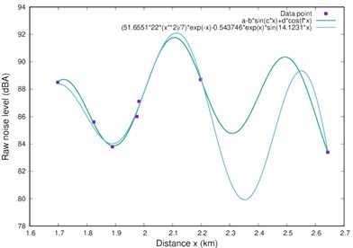
where the parameters , and may respectively be taken as the noise strength and the amplitudes in dBA while and are the corresponding wave numbers calculated in per kilometers. For example, the best fit parameter for the Morning take off data are: 74.1031±1.6980 dBA, –3.4260±0.2802 dBA, –14.3289±1.9280 dBA, 15.6808±0.0296 km-1, and 1.4421±0.0141 km-1. This is compared with the best fit of Eq. (1) in Fig. 2(c). Even though the two functions give comparable fit to the data we see that their differences clearly manifest in the long distance range.
Table 1Best fit values for the parameters of the nonlinear model function. Note that parameter a = 1 dBAkm-1
Morning | Afternoon | Evening | ||||
Parameter | ASE | ASE | ASE | |||
51.6551 | +/–0.0913 (0.18 %) | 52.1962 | +/–0.3352 (0.64 %) | 52.0684 | +/–0.5903 (1.14%) | |
14.1119 | +/–0.0199 (0.14 %) | 13.9874 | +/–0.1110 (0.79%) | 14.1044 | +/–0.3002 (2.13 %) | |
–0.5437 | +/–0.0407 (7.48 %) | -0.5063 | +/–0.1338 (26.44 %) | –0.2471 | +/–0.2629 (106 %) |
Fig. 1Fitted plot of the raw data for the a) morning take-off, b) afternoon, c) evening data
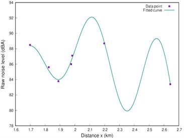
a)
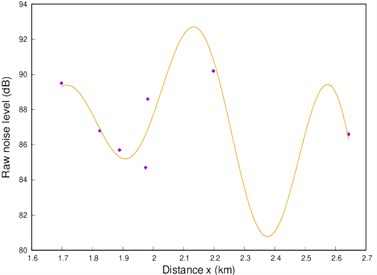
b)
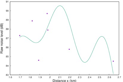
c)
4. Discussion
Our results show a noise model function characterized by a noise level that slowly dissipates with distance. The noise level which grows quadratically with the radial distance from the runway is attenuated exponentially by some physical factors over the radial distance. The sinusoidal propagation over the spatial distance in the atmospheric medium is characteristic of the sound waves. The parameter ‘’ is understood as the predicted noise strength at the radial distances corresponding to or larger than that of the minimum circular area around the source point. The overall effect of both components of the model function is a shifted sinusoidal wave function with varying amplitude and whose peak-to-peak strength is defined by the noise strength per unit area and the attenuation factor. We note that this is only defined for a radial distance greater than or equal to the closest distance of measure to the runway corresponding to a minimum circular area. Thus, the model function cannot be used to estimate the maximum noise generated at the source point but may be used to infer the extent to which the noise level is within the required threshold.
4.1. Relative behavior of the take-off parameter fits
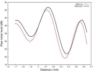
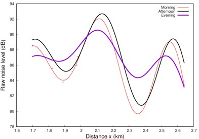
A superimposed data plots in Fig. 2 show a clear pattern of a sinusoidal waveform characteristic of sound waves. Given the external physical factors, the aircraft raw noise level strength during morning take-off flights, assuming all other things being equal, would be lower than it would be in the afternoon due to the temperature difference. Similarly, the noise propagation is also expected to be slower in the morning than for the afternoon. This is supported by the plots in Fig. 2(a), where the crest points for morning noise level at different distances are not only lower than for the afternoon but also lags behind when the temperature of the surrounding area was significantly higher than in the morning time. The same explanation holds for the trough point. In addition, the afternoon noise level is further enhanced by the possible increase in the background noise due to the increased human activities and other forms of transportation within the environment of the airport.
In Fig. 2(b) the evening plot is at significant variance with morning and afternoon data plots. This is understood as the effect of the sharp drop in both the temperature and the background noise level in the evening. Fig. 2(c) shows the comparison of both model functions of Eqs. (1) and (2) with respect to the experimental data points.
Fig. 2Plots for a) morning and afternoon take-offs, and b) morning, afternoon and evening take-offs, c) comparison of the model functions in Eqs. (1) and (2) with the data for morning take-offs
a)
b)
c)
4.2. Prediction of the minimum distance for noise thresholds
The negative health effects of aircraft noise levels from proximate locations to airports become pronounced around the world. Residential land use should, therefore, be planned and situated with thorough considerations of airport noise and its potential risks [11]. Consideration for a safe distance between residential zones and airport locations is thus necessary. Numerical solution of the model function is used to predict the minimum distance for the locations of residential buildings or public institutions from the airport using the thresholds from earlier studies [6]. We predict the minimum radial distance for the 40 dBA, 45 dBA and 50 dBA thresholds. The minimum distance of approximately 3.60 km, 3.64 km and 4.04 km are thus predicted as the safe limits from the morning, afternoon and evening take-off data. Remarkably the predicted distance increase with decreasing noise level for each of the models fits. The trend of the predicted values shows increasing distance for a fixed noise threshold from the morning to evening model fits. Urban residents could actually receive up to 45 dBA of noise without complaint, while it is 40 dBA (suburban residents) and lower at 35 dBA for rural residents. In fact [14] show that a distance of 3 km to the side of the flight paths calls for concerns. The authors further show that approximately 3.8 km distance is required for a 55 dBA thresholds for a noise abatement zone that requires aircraft to be higher than 1.5 km above the ground level before flying residential areas.
5. Conclusion
This paper shows that the minimum safe distance from a morning aircraft take-off noise level of about 45 dBA thresholds for urban residents with limited complaints or minimum potential health hazard is about 3.6 km. The minimum safe distance increases to 3.64 km in the afternoon, and 4 km in the evening. We consider the minimum safe distance in the evening as a standard minimum for situating airport away from residential houses. We conclude that our proposed model function for aircraft take-off noise prediction with distances radially from a runway could be used to predict safe distance for different aircraft noise levels and thresholds. Further studies which effectively capture information of the aircrafts and flight pattern and paths is expected to provide a more robust predictive model.
References
-
Getzner M., Zak D. Health Impacts of Noise Pollution Around Airports: Economic Valuation and Transferability. Environmental Health – Emerging Issues and Practice, 2012.
-
Rodrigue J. P., Comtois C., Slack B. The Geography of Transport System. Routledge, Taylor and Francis Group, London, 2006.
-
Clark C., Stansfeld S. A. The effect of transportation noise on health and cognitive development: a review of recent evidence. International Journal of Comparative Psychology, Vol. 20, Issues 2-3, 2007, p. 145-158.
-
Lu C., Morrell P. Determination and applications of environmental costs at different sized airports – aircraft noise and engine emissions. Transportation, Vol. 33, Issue 1, 2006, p. 45-61.
-
Stansfeld S. A., Clark C., Cameron R. M., Alfred T., Head J., Haines M. M., Van Kamp I., Van Kempen E., Lopez Barrio I. Aircraft and road traffic noise exposure and children’s mental health. Journal of Environmental Psychology, Vol. 29, Issue 2, 2009, p. 203-207.
-
Babisch W., Van Kamp I. Exposure-response relationship of the association between aircraft noise and the risk of hypertension. Noise and Health, Vol. 11, Issue 44, 2009, p. 161-168.
-
Eriksson C., Rosenlund M., Pershagen G., Hilding A., Östenson C. G., Bluhm G. Aircraft noise and incidence of hypertension. Epidemiology, Vol. 18, Issue 6, 2007, p. 716-721.
-
Van Kempen E., Van Kamp I., Lebret E., Lammers J., Emmen H., Stansfeld S. Neurobehavioral effects of transportation noise in primary schoolchildren: a cross-sectional study. Environmental Health, Vol. 9, 2010, p. 25.
-
Haines M. M., Stansfeld S. A., Job R. F., Berglund B., Head J. Chronic aircraft noise exposure, stress responses, mental health and cognitive performance in school children. Psychological Medicine, Vol. 31, Issue 2, 2001, p. 265-277.
-
Airport Planning Manual Part 2: Land Use and Environmental Control. Third Edition, ICA, Doc 9104 AN/902, 2002
-
Dunn D. G., Peart N. A. Aircraft Noise Source and Contour Estimation. National Aeronautics and Space Administration, Washington, DC20546, Report No. NASA CR-114649, 1973.
-
Bates D. M., Watts D. G. Nonlinear Regression Analysis and Its Application. John Wiley and Sons, 1988.
-
Marquardt D. W. An algorithm for least-squares estimation of nonlinear parameters. Journal of the Society for Industrial and Applied Mathematics, Vol. 11, Issue 2, 1963, p. 431-441.
-
Burgess M., Mccarty M. Monitoring aircraft noise levels to the side of flight paths. Acoustics Australia, Vol. 38, Issue 2, 2010, p. 63-68.
Cited by
About this article

The authors would like to thank Ms. Ilse Gayl for her kind financial support.
