Mathematical modeling of first order process with dead time using various tuning methods for industrial applications

Shanmugam, Sathish Kumar; Duraisamy, Yuvaraj; Ramachandran, Meenakumari; Arumugam, Senthilkumar

doi:10.21595/mme.2019.20447

Mathematical Models in Engineering

Browse Journal

Submit article

Published: 31 March 2019

Check for updates

Mathematical modeling of first order process with dead time using various tuning methods for industrial applications

Sathish Kumar Shanmugam¹

Yuvaraj Duraisamy²

Meenakumari Ramachandran³

Senthilkumar Arumugam⁴

¹Jansons Institute of Technology, Coimbatore, Tamilnadu, India

²Tamilnadu College of Engineering, Coimbatore, Tamilnadu, India

³Kongu Engineering College, Erode, Tamilnadu, India

⁴Chettinad College of Engineering and Technology, Karur, Tamilnadu, India

Corresponding Author:

Sathish Kumar Shanmugam

Cite the article Download PDF

Downloads 1883

CrossRef Citations 2

Abstract

The proposed research involves Mathematical modeling for first order process with dead time using various tuning methods for industrial applications. Different tuning methods are proposed. Proposed method selection depends on plant operating conditions and also depending upon the process dynamics. The PID controller is most widely used for industrial process control. Modeling were developed for modified internal control model [4-6] in this proposed research. The proposed work is the modeling and simulation of three different first order processes with dead time. The standard controller tuning method is used to obtain the steady state response of first order with dead time.

Mathematical modeling of first order process with dead time using various tuning methods for industrial applications

Highlights

The controller tuning is performed to stabilize the process output according to the set point changes.
The controller tuning is based on the error signal and it is performed to nullify the error.
The feed-forward controller takes control action according to the load changes.
Dead time is the time taken by the system to produce the response after the input is applied

1. Introduction

The preferred output of a control system is obtained by tuning the controller parameters according to the set point. The first order system is widely used in industrial control system to represent the behavior of process dynamics [1, 2]. The delay takes place in process measurement, controller action, actuator operation and computation is called delay time. Dead time is the time taken by the system to produce the response after the input is applied [3].

2. Block diagram of feedback control system

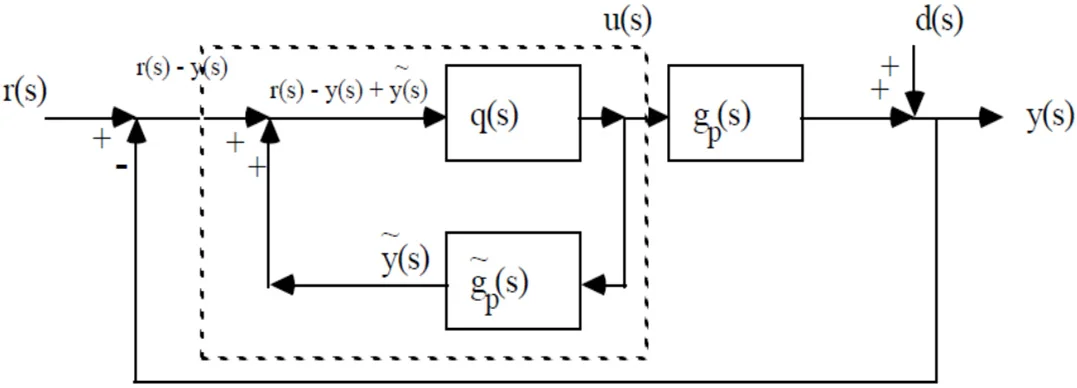
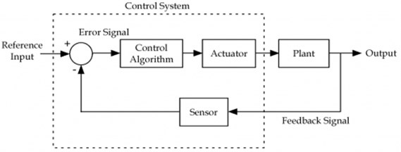
Fig. 1 shows the block diagram proposed IMC Feedback Control System. The algorithm is necessity $o e$ for tuning. The control action is done by the actuator. The input signal which is attenuated will control the parameter. Sensor is used for controlling the signal measure the process variable from the process output. The control algorithm is used to nullify the error signal to zero [4-6].

Fig. 1Block diagram of proposed IMC feedback control system

3. Literature review

• Astrom and Haggland proposed an alternative method of the system. The technique itself create its own test signal based on the estimation [7].

• The robustness of the automatic tuning of controller by Zeigler’s technique is improved by Astrom and Haggland method. In this robust loop shaping rule called MIGO and AMIGO is introduced. MIGO concentrates on maximizes the integral gain to improve the robustness of the system.

• Wallen et al., enhanced the loop shaping based tuning by introducing an additional constraint the ratio of integral time to the derivative time for tuning the PID controller. And also, it makes some conditions the curvature should be negative and it should have a decreasing phase of a curve.

• Zeigler and Nichols proposed the first auto tuning procedure for controllers. The sensitivity, Reset rate and pre-act time are the characteristics of the reaction curve for designing an automatic controller [8, 9].

4. Materials and methods

4.1. Controller tuning

When PID controller has been selected, Different methods are required for tuning. This is called as ‘controller tuning’. Different methods adopted for the proposed tuning are analysed and its results were carried out with the modified structure. The method proposed is Internal Model Control (IMC).

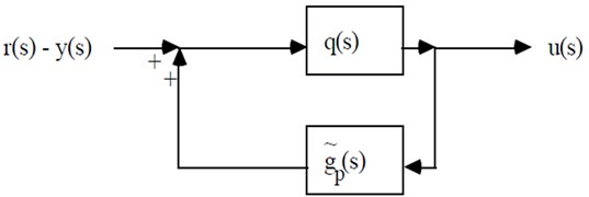
Fig. 2Proposed IMC schematic circuit

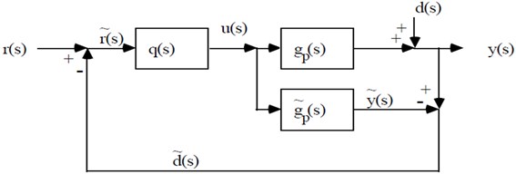
Fig. 3Proposed IMC schematic circuit with surface change

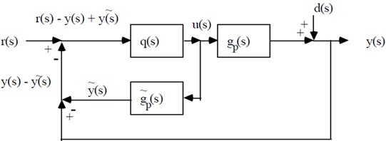
Fig. 4Modified proposed IMC schematic circuit with surface change

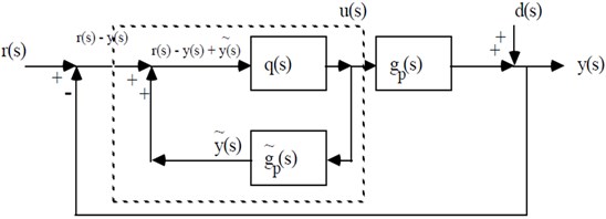
Fig. 5Modified proposed IMC schematic circuit with surface change inner loop

The standard feedback of proposed IMC circuit is given by:

1

g_{c} (s) = \frac{q (S)}{1 - g_{p} (s) q (S)} .

The equivalent circuit equation of proposed structure IMC is given by:

2

g_{c} (s) = \frac{q (S)}{1 - {\tilde{g}}_{p} (s) q (S)} .

The PID controller tuning equation is given by:

3

g_{c} (s) = k_{c} [\frac{τ_{1} τ_{D} s^{2} + τ_{1} s + 1}{τ_{1} s}] [\frac{1}{τ_{F} s + 1}] .

The proposed method first order process is given by:

4

{\tilde{g}}_{p} (s) = \frac{k_{p}}{τ_{p} s + 1} .

After filtering in the process is given by:

5

q (s) = \tilde{q} (s) f (s) = {g_{p}}^{- 1} (s) f (s) = [\frac{τ_{p} s + 1}{k_{p}}] [\frac{1}{λ_{s} + 1}], q (s) = \frac{1}{k_{p}} \frac{τ_{p} s + 1}{λ_{s} + 1},

After transforming the equation can be written as:

6

g_{c} (s) = \frac{q (S)}{1 - {\tilde{g}}_{p} (s) q (S)} = \frac{\frac{τ_{p} s + 1}{k_{p} {(λ}_{s} + 1)}}{1 - \frac{k_{p}}{τ_{p} s + 1} \frac{τ_{p} s + 1}{k_{p} {(λ}_{s} + 1)}} = \frac{τ_{p} s + 1}{k_{p} λ_{s}} .

Multiplying with tuning parameters:

7

g_{c} (s) = [\frac{τ_{p}}{k_{p} λ}] \frac{τ_{p} s + 1}{τ_{p} s} .

Similarly, for second order process:

8

g_{c} (s) = [\frac{τ_{1} + τ_{2}}{k_{p} λ}] [\frac{τ_{1} τ_{2} s^{2} + (τ_{1} + τ_{2}) s + 1}{(τ_{1} + τ_{2}) s}] .

4.2. Methods of tuning for servo response

The controller tuning is performed to stabilize the process output according to the set point changes. The feedback controller is used for setting point tracking. The error signal is generated which is the differences between setpoint and process variable. The controller tuning is based on the error signal and it is performed to nullify the error. The controller tuning is performed to stabilize the process output according to the load disturbance. The feedback controller is not suitable for load disturbance tracking. The advanced control mechanism such as feedforward controller is used to track the load disturbance. The feedforward controller takes control action according to the load changes.

4.2.1. Cohen-Coon tuning

This method is also based on a delayed first order rise, and the method tunes the PID gains to achieve quarter-amplitude damping, i.e. each peak in the transient is one quarter of the immediate preceding peak. If the unit step response of the open loop plant is available, then process gain ( $K$ ), dead time ( $t_{d}$ ) and time constant ( $T$ ) can be determined. PID controllers are designed to test the system and selected based on the performance and selection criteria. Table 1 shows the Cohen Coon method.

Table 1Cohen Coon

Controller type	( $K_{C}$ )	$T_{I}$	$T_{D}$
PID	$\frac{1.49}{k_{m} τ_{m}}$	2 $τ_{m}$	$1.27 τ_{m}$

4.2.2. Ziegler Nichols tuning

Ziegler Nichols method is also called as Ultimate Cycle Method. It is based on adjusting a closed loop until steady state oscillations occur. This method is used to minimizing the total error of the response. To return to desired level operation as soon as possible and to keep the maximum deviation as small as possible this method is used. The integral absolute error is the integral error which defines the stability of the system. Larger the integral error, smaller the stability is. Thus, by minimizing the integral absolute error we get the good robustness and performance. Thus, IAE is also taken measuring parameter. Control objectives focus on the behavior of the system such as to produce a zero steady state error, a fast transient response to a step command, a short settling time and low overshoot. It is also desirable to make the system less sensitive to disturbance. The period of these oscillations is defined as the ultimate period $P_{u}$ . The controller gains at which these oscillations occur is referred to as the ultimate gain $K_{u}$ . Ziegler Nichols method are shown in Table 2.

Table 2Ziegler Nichols method

Controller type	$K_{C}$	$T_{I}$	$T_{D}$
PID Zeigler Nichol’s	$\frac{K_{u}}{1.7}$	$\frac{P_{u}}{2}$	$\frac{P_{u}}{8}$
Ultimate cycle PID developed by mc Millan	$1.009 \frac{T m}{k m τ_{m}} {\{\frac{1}{1 + {(\frac{T m}{τ_{m}})}^{. 65}}\}}^{2}$	$2 τ_{m} \{1 + {(\frac{T m}{τ_{m}})}^{. 65}\}$	0.26 $T_{I}$

4.2.3. FOPTD transfer functions

The PID tuning formulas are applied for the three FOPTD transfer functions to obtain the analysis. The FOPTD transfer function is considered based on ratio of dead-time to the time constant less than one, equal to 1 and greater than 1. Z-N method is time consuming and forces the system to margin if instability. Many other algorithms have been proposed to solve these problems by obtaining critical data (ultimate gain and frequency) under more acceptable conditions. One of these methods is damped oscillation method. Z-N method are shown in Table 3.

Table 3Z-N method

Controller type	$K_{C}$	$T_{I}$	$T_{D}$
PID	$K_{u} / 1.3$	$2.2 P_{u}$	$P_{u} / 5.2$

The implicit manner based PID control algorithm is simple and robust to handle the model inaccuracies and hence using IMC-PID tuning method a clear trade-off between closed loop performance with damped oscillation and robustness to model inaccuracy is achieved with a single tuning parameter are show in Table 4 for implicit manner.

Table 4For implicit manner

Controller type	$K_{C}$	$T_{I}$	$T_{D}$
PID	$2 / K (λ + θ / 2)$	2 $λ + θ$	$\frac{λ θ + (θ^{2}) / 4}{2 T + θ}$

4.2.4. Integrating process transfer functions

The PID tuning formulas are applied for the three different order transfer functions to obtain the analysis in order to study the integrating process performance. The different order integrating process transfer functions considered for the analysis are.

The PID tuning formulas are applied for the three different order transfer functions to obtain the analysis in order to study the integrating process performance. The different order integrating process transfer functions considered for the analysis are,

(i) Transfer function 1.

The pure integrator process transfer function with low delay consider as example of benchmark process default value of second order system for controlling:

9

G_{p 1} (s) = \frac{1}{s} e^{- 2 s} .

(ii) Transfer function 2.

The pure integrator process transfer function with low delay consider as example of benchmark process default value of second order system for controlling:

10

G_{p 2} (s) = \frac{1}{s} e^{- 5 s} .

(iii) Transfer function 3.

The higher order integrator process transfer function without delay consider as example of benchmark process default value of second order system for controlling:

11

G_{p 3} (s) = \frac{{(0.17 s + 1)}^{2}}{s {(s + 1)}^{2} (0.028 s + 1)} .

The transfer function is approximated to integrator process with delay by using half rule approximation in order to work with, and the transfer function is example of benchmark process default value of second order system for controlling:

12

G_{p 3} (s) = \frac{1}{s} e^{- 1.69 s} .

5. Results and discussions

5.1. MATLAB software for simulation of FOPDT

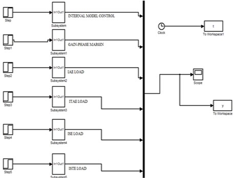
Simulink is widely used for analysis of first order process with dead time. The Simulink is used in this proposed work to obtain the response of first order with dead time. Simulink block diagram of FOPTD set point and transfer function for load disturbance are shown in Figs. 6 and 7.

Fig. 6Simulink block diagram for FOPTD for set point

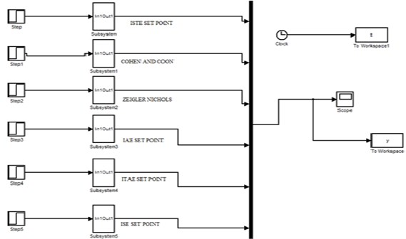
Fig. 7Simulink block diagram of FOPTD transfer function for load disturbance

5.1.1. Transfer function 1

The ratio of time delay $θ$ to the time constant $τ$ is less than one:

13

G_{p 1} (s) = \frac{1}{5 s + 1} e^{- s} .

Fig. 8 shows the output of transfer function 1. Fig. 11 shows the output of transfer function 1 setpoint.

Fig. 8Output of transfer function 1

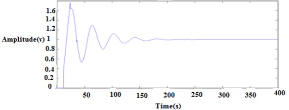
5.1.2. Transfer function 2

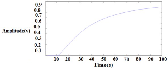
The ratio of time delay $θ$ to the time constant $τ$ is unity:

14

G_{p 2} (s) = \frac{4}{10 s + 1} e^{- 10 s} .

Fig. 9 shows the output of transfer function 2. Fig. 12 shows the output of transfer function 2 setpoint.

Fig. 9Output of transfer function 2

5.1.3. Transfer function 3

The ratio of time delay $θ$ to the time constant $τ$ is greater than one:

15

G_{p 3} (s) = \frac{1}{7 s + 1} e^{- 14 s} .

Fig. 10 shows the output of transfer function 3. Fig. 13 shows the output of transfer function 3 setpoint.

Fig. 10Output of transfer function 3

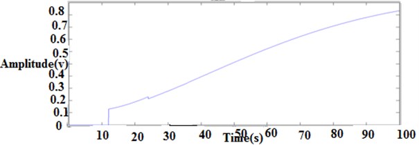
Fig. 11Output of transfer function 1 (set point)

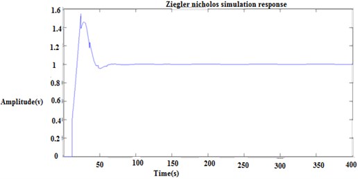
Fig. 12Output of transfer function 2 (set point)

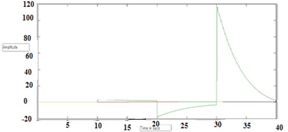
Fig. 13Output of transfer function 3 (set point)

5.2. Simulation results of closed loop methods

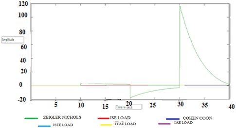
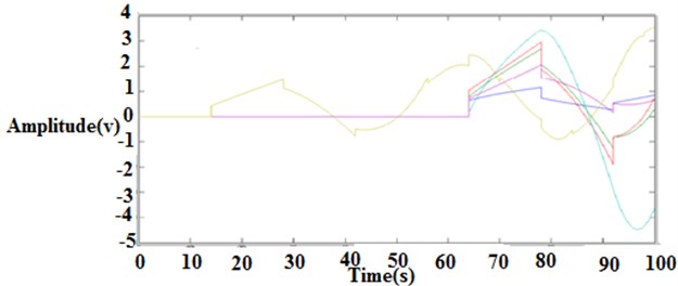
The various output loop response is shown in Figs. 14 to 18.

Fig. 14Ziegler Nichols closed loop response

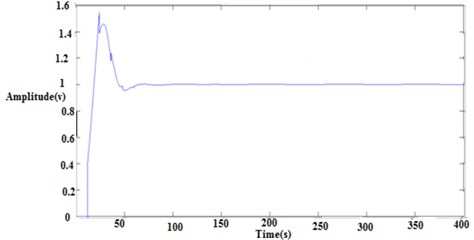
Fig. 15IMC closed loop response

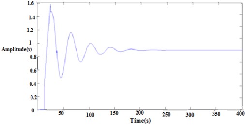
Fig. 16Integral of square error closed loop response

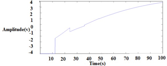
Fig. 17Integral of absolute error closed loop response

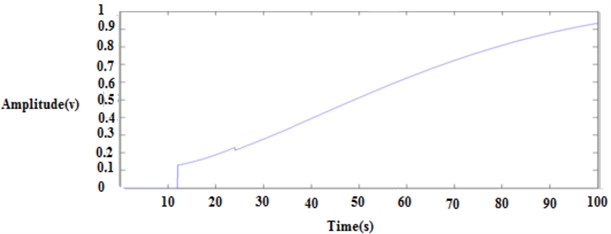
Fig. 18Integral of square time error closed loop response

6. Conclusions

The first order with delay process is widely used to represent the process dynamics. The selection of controller and tuning methods are important consideration in the control system design. This proposed work is the tuning and analysis of three different first order with dead time. This analysis shows that the performance is best for the ratio less than 1 for Zeigler Nichols, Cohen coon, ITAE load disturbances and IMC, ITAE, ISE, ISTE, GP set point method. This model produces a better transient response. This proposed work can be extended by using Fuzzy Logic Controller for first order with dead time and performance characteristics can be compared.

References

Ozipneci Burak, Tolbert Leon M. Simulink implementation of induction machine model – a modular approach. IEEE International Electric Machines and Drives Conference, 2003.

Publisher
Dorf C. R., Bishop R. F. Modern Control System. 10th Edition, Prentice Hall, 2005.

Search CrossRef
Dumitrescu A., Fodor D., Jokinen T., Rosu M., Bucurencio S. Modeling and simulation of electric drive system using Matlab/Simulink environment. International Conference on Electric Machines and Drives (IEMD), 1999, p. 451-453.

Publisher
Le Huy H. Modeling and simulation of electrical drives using Matlab/Simulink and power system block set. 27th Annual Conference of the IEEE Industrial Electronics Society, 2001.

Search CrossRef
Nizam Kamarudin M., Rozali Sahazati Md. Implementation of cascade control DC motor. International Conference on Power and Energy, 2008.

Search CrossRef
Sondhi S., Hote Y. V. Fractional order PID controller for load frequency control. Energy Conversion and Management, Vol. 85, 2014, p. 343-353.

Publisher
Debbarma S., Dutta A. Utilizing electric vehicles for LFC in restructured power systems using fractional order controller. IEEE Transactions on Smart Grid, Vol. 8, Issue 6, 2017, p. 2554-2564.

Publisher
De Keyser R., Muresan C. I., Ionescu C. M. A novel auto-tuning method for fractional order PI/PD controllers. ISA Transactions, Vol. 62, 2016, p. 268-275.

Publisher
Moosavi S. H. S., Bardsiri V. K. Satin bowerbird optimizer: a new optimization algorithm to optimize ANFIS for software development effort estimation. Engineering Applications of Artificial Intelligence, Vol. 60, 2017, p. 1-15.

Publisher

Cited by

Conventional and Fuzzy Control for First Order Plus Dead Time Process Using Different Tuning Methods

Khalid M Mousa Al-zobai | Dalya S Makki

(2021)

Study cases methodology in process dynamic and industrial plants control subject

Ana M. Borreguero | Jesus M. García‐Vargas | Luz Sánchez‐Silva | Ana R. Osa

(2020)

About this article

Received

12 December 2018

Accepted

27 January 2019

Published

31 March 2019

DOI

https://doi.org/10.21595/mme.2019.20447

Keywords

IMC

tuning

transfer function

simulation

analysis

This is an open access article distributed under the Creative Commons Attribution License, which permits unrestricted use, distribution, and reproduction in any medium, provided the original work is properly cited.

Next article in issue Next

Research article

2022 06 30

A comparative analysis of different approaches used for modelling and solving differential equations in Simulink/MATLAB

Pankaj Mohindru, Pooja Mohindru

Research article

2019 12 31

Graphical PID tuning method for uncertain fractional-order multivariable systems

Minghui Chu, Chi Xu, Jizheng Chu

Research article

2018 02 15

State feedback based fractional order control scheme for linear servo cart system

Ibrahim Mustafa Mehedi

Research article

2017 10 21

Analytical method of designing a comparable milling machine model based on Matlab/Simulink

Bashir Osman, Haitao Zhu

S. K. Shanmugam, Y. Duraisamy, M. Ramachandran, and S. Arumugam, “Mathematical modeling of first order process with dead time using various tuning methods for industrial applications,” Mathematical Models in Engineering, Vol. 5, No. 1, pp. 1–10, Mar. 2019, https://doi.org/10.21595/mme.2019.20447

Copy Extrica

Copied to clipboard!

TY  - JOUR
DO  - 10.21595/mme.2019.20447
UR  - https://doi.org/10.21595/mme.2019.20447
TI  - Mathematical modeling of first order process with dead time using various tuning methods for industrial applications
T2  - Mathematical Models in Engineering
AU  - Shanmugam, Sathish Kumar
AU  - Duraisamy, Yuvaraj
AU  - Ramachandran, Meenakumari
AU  - Arumugam, Senthilkumar
PY  - 2019
DA  - 2019/03/31
PB  - JVE International Ltd.
SP  - 1-10
IS  - 1
VL  - 5
SN  - 2351-5279
SN  - 2424-4627
ER  - 

Copy Ris

Copied to clipboard!

@article{Shanmugam_2019,
	doi = {10.21595/mme.2019.20447},
	url = {https://doi.org/10.21595/mme.2019.20447},
	year = 2019,
	month = {mar},
	publisher = {{JVE} International Ltd.},
	volume = {5},
	number = {1},
	pages = {1--10},
	author = {Sathish Kumar Shanmugam and Yuvaraj Duraisamy and Meenakumari Ramachandran and Senthilkumar Arumugam},
	title = {Mathematical modeling of first order process with dead time using various tuning methods for industrial applications},
	journal = {Mathematical Models in Engineering}
}

Copy Bibtex

Copied to clipboard!

[1]S. K. Shanmugam, Y. Duraisamy, M. Ramachandran, and S. Arumugam, “Mathematical modeling of first order process with dead time using various tuning methods for industrial applications,” Mathematical Models in Engineering, vol. 5, no. 1, pp. 1–10, Mar. 2019, doi: 10.21595/mme.2019.20447.

Copy IEEE

Copied to clipboard!

Shanmugam, Sathish Kumar, Yuvaraj Duraisamy, Meenakumari Ramachandran, and Senthilkumar Arumugam. “Mathematical Modeling of First Order Process with Dead Time Using Various Tuning Methods for Industrial Applications.” Mathematical Models in Engineering 5, no. 1 (March 31, 2019): 1–10. https://doi.org/10.21595/mme.2019.20447.

Copy Chicago

Copied to clipboard!

Mathematical modeling of first order process with dead time using various tuning methods for industrial applications

Abstract

Highlights

1. Introduction

2. Block diagram of feedback control system

3. Literature review

4. Materials and methods

4.1. Controller tuning

4.2. Methods of tuning for servo response

4.2.1. Cohen-Coon tuning

4.2.2. Ziegler Nichols tuning

4.2.3. FOPTD transfer functions

4.2.4. Integrating process transfer functions

5. Results and discussions

5.1. MATLAB software for simulation of FOPDT

5.1.1. Transfer function 1

5.1.2. Transfer function 2

5.1.3. Transfer function 3

5.2. Simulation results of closed loop methods

6. Conclusions

References

Cited by

About this article

Related Articles