Dynamic modeling and simulation of three-member robot manipulator

Mickoski, Hristijan; Mickoski, Ivan; Djidrov, Marjan

doi:10.21595/mme.2018.20319

Mathematical Models in Engineering

Browse Journal

Submit article

Published: 31 December 2018

Check for updates

Dynamic modeling and simulation of three-member robot manipulator

Hristijan Mickoski¹

Ivan Mickoski²

Marjan Djidrov³

^{1, 2, 3}Faculty of Mechanical Engineering in Skopje, Ss. Cyril and Methodius University in Skopje, 1000 Skopje, Republic of Macedonia

Corresponding Author:

Ivan Mickoski

Cite the article Download PDF

Downloads 1644

Abstract

Dynamic model analysis of manipulator as mechanical structure is presented for further purpose in actuator selection and process for establishing control strategy. Control problems involves determination of control forces and moments applied in manipulator joints that will ensure movements along a certain defined trajectory. Trajectory design is the basis for the manipulator control process. This problem is quite complex because the manipulator is a connected system in which the movement of a member affects the movement of other. Therefore, in following is presented a method for forces and moments determination in kinematic joints of a three-member manipulator analytically and also by using simulation dynamical model in the Matlab/Simulink program package. The friction forces in the kinematics joints are not taken into account.

1. Introduction

In order to study and analyse the mechanical or electrical systems, standard method is through their modelling. By modelling a system, an adequate faithful model of the system is created and there are many definitions of term system model. Modelling is a process of organized knowledge of a given system, which is the most important stage in the research of a single system. The modelling process also involves a process of simulation, which is a method of conducting experiment on the model. The model obtained through modelling includes basic properties of the system which are necessary for solving research problems. One of the reasons for creating a model is to answer control system problems. Mathematical models or computer models are created for studying manipulators. Mathematical models refer to a system of mathematical equations and expressions basis on hypotheses and theories in the field of mechanics, physics, etc. The computer simulated models are the same as mathematical models but are formed in another language other than the normal language of mathematics.

The dynamics of the robot manipulator defines the relationship between the forces, i.e. joint moments brought by the actuators and the equations of motion. Dynamic analysis are the most important task because they are closest for describing actual situation of moving systems. Two types of problems are in dynamics analysis [1], the first is forward problem which refers to determine the forces that cause movement for a given laws of motion, and second is inverse problem [2] for computing forces and/or moments based on the kinematics of a body. The robot model developed will not only help in understanding the dynamic behavior but also allow to integrate data acquisition, control, etc. to generate a virtual robot. Such virtual robot in turn may also be used as a training tool if connected with an external device like the robots teach pendant [3, 4].

For analysis of loads of mechanical systems element under the effect of given external and inertial forces from members movements, the kinetostatics method is used. This method is based on the D’Alembert’s principle which states that, the forces acting to a given body and inertial forces from the movement are in a fictitious balance. This method makes it possible to use lows for static reduction and equilibrium in dynamic analysis associated with inertial forces which often determine the strength, longevity, and reliability of modern structures.

The robot manipulator is considered as a system of rigid bodies with defined masses and its own inertial moments, mechanical model of two link manipulator can be found in [5]. The Effect of different sets of initial and boundary conditions on the joints torques is investigated in [6] and control simulation of two link robot manipulator to get the desired position by using computed torque control method is presented in [7]. The combination of Matlab and Simulink is proposed in [8], the method allows to manipulate the robotic system and to visualize the robot’s behavior from different perspectives. The D-H method is used in [9] to establish a connecting rod coordinate system of six-degree-of-freedom moving robot and combined with Solid Works and ADAMS is simulated the moving robot to verify the correctness of the kinematic model.

Equations that define the model dynamics of the robot manipulator are ordinary differential equations where variables are components of position and velocity vectors. These equations are obtained using the Newton-Euler or by Lagrange method which is applied and presented in following. Using the Lagrangian method for any system, a system of n nonlinear second-order equations is obtained in the following form:

1

\frac{d}{d t} [\frac{\partial E_{k}}{\partial {\dot{q}}_{i}}] - \frac{\partial E_{k}}{\partial q_{i}} = Q_{i}, i = 1,2, \dots, n .

The number of system equations $n$ is determined by the number of generalized coordinate $q_{i}$ which can describe the movement of the system.

Further, the possible displacements of each of the joints are considered individually, and by using the principle of virtual work, equations for each joint are written in the following form:

2

\sum δ A_{i} = Q_{i} {δ φ}_{i} .

By equalizing the two obtained equations for each joint, control moments and forces are obtained. For kinetostatic analysis of the robot manipulator, Lagrange equation and principle of virtual work will be presented. The objective of this paper is to present a method for forces and moments determination in kinematic joints of a three-member manipulator analytically and also by using simulation dynamical model in the Matlab/Simulink program package.

2. Manipulator characteristics

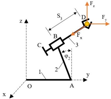
For determination of control force and moment, three-member manipulator from Fig. 1 will be used. Equations of motion of the manipulator are:

3

φ_{2} = - 0.4 {c o s}^{2} (\frac{π t}{2}) [r a d], S_{3} = 1.2 - 8 t^{3} [m], t = 0.5 [s] .

Dimensions of manipulator member are: $l_{1} =$ 0.9 m, $l_{2} =$ 0.5 m, $l_{3} =$ 0.7 m. External forces on the manipulator are: $F_{x} =$ 2 N, $F_{y} =$ –3 N, $F_{z} =$ 4 N and cross section area is $A =$ 1 cm².

3. Manipulator kinetostatic analysis by Lagrange’s equation and principle of virtual work

The second-order Lagrange’s equation for the manipulator:

4

\frac{d}{d t} [\frac{\partial E_{k}}{\partial {\dot{φ}}_{2}}] - \frac{\partial E_{k}}{\partial φ_{2}} = Q_{1}, \frac{d}{d t} [\frac{\partial E_{k}}{\partial {\dot{S}}_{3}}] - \frac{\partial E_{k}}{\partial S_{3}} = Q_{2} .

where $Q_{1}$ and $Q_{2}$ are generalized motion forces, respectively to generalized coordinates $q_{1}$ and $q_{2}$ . Generalized coordinates are:

5

q_{1} = φ_{2} = - 0.4 {c o s}^{2} (\frac{π t}{2}) [r a d], q_{2} = S_{3} = 1.2 - 8 t^{3} [m] .

Fig. 1Three-member manipulator

Manipulator kinetic energy which include kinetic energy of all manipulator members, is given by equation:

6

E_{k} = \sum E_{K_{i}} = {E_{k}}_{1} + {E_{k}}_{2} + {E_{k}}_{3} .

where for $E_{k 1} =$ 0 manipulator kinetic energy is sum of kinetic energy of member 2 and 3. Member 2 makes rotation with angular velocity ${\dot{φ}}_{2}$ , and kinetic energy is:

7

{E_{k}}_{2} = \frac{J_{x 2} ω_{2}^{2}}{2} = \frac{m_{2} {l_{2}}^{2} {\dot{φ}}_{2}^{2}}{3 ∙ 2},

where $J_{x 2} = m_{2} {l_{2}}^{2} / 3$ and $ω_{2} = {\dot{φ}}_{2} .$

Member 3 makes translation with velocity ${\dot{S}}_{3}$ , and kinetic energy is:

8

{E_{k}}_{3} = \frac{m_{3} {V_{C_{3}}}^{2}}{2} = \frac{m_{3}}{2} [{(l_{2} {\dot{φ}}_{2})}^{2} + {({\dot{S}}_{3})}^{2}],

where:

9

V_{C_{3}} = {\dot{X}}_{C_{3}}^{2} + {\dot{Y}}_{C_{3}}^{2} + {\dot{Z}}_{C_{3}}^{2} = {(- {\dot{S}}_{3})}^{2} + {(- l_{2} {\dot{φ}}_{2} c o s φ_{2})}^{2}

+ {(- l_{2} {\dot{φ}}_{2} s i n φ_{2})}^{2} = {(l_{2} {\dot{φ}}_{2})}^{2} + {({\dot{S}}_{3})}^{2} .

The total kinetic energy is:

10

E_{k} = \frac{1}{2} (a {\dot{φ}}_{2}^{2} + b {\dot{S}}_{3}^{2}),

where $a = m_{2} / 3 + m_{3}$ and $b = m_{3} .$

We compute the partial derivatives of kinetic energy in terms of generalized coordinates:

11

\frac{\partial E_{k}}{\partial {\dot{φ}}_{2}} = \frac{\partial}{\partial {\dot{φ}}_{2}} [\frac{1}{2} (a {\dot{φ}}_{2}^{2} + b {\dot{S}}_{3}^{2})] = a {\dot{φ}}_{2},

\frac{\partial E_{k}}{\partial φ_{2}} = \frac{\partial}{\partial φ_{2}} [\frac{1}{2} (a {\dot{φ}}_{2}^{2} + b {\dot{S}}_{3}^{2})] = 0,

\frac{d}{d t} [\frac{\partial E_{k}}{\partial {\dot{φ}}_{2}}] = \frac{d}{d t} (a {\dot{φ}}_{2}) = a {\ddot{φ}}_{2},

and velocities:

12

\frac{\partial E_{k}}{\partial {\dot{S}}_{3}} = \frac{\partial}{\partial {\dot{S}}_{3}} [\frac{1}{2} (a {\dot{φ}}_{2}^{2} + b {\dot{S}}_{3}^{2})] = b {\dot{S}}_{3},

\frac{\partial E_{k}}{\partial S_{3}} = \frac{\partial}{\partial S_{3}} [\frac{1}{2} (a {\dot{φ}}_{2}^{2} + b {\dot{S}}_{3}^{2})] = 0,

\frac{d}{d t} [\frac{\partial E_{k}}{\partial S_{3}}] = \frac{d}{d t} (b {\dot{S}}_{3}) = b {\ddot{S}}_{3} .

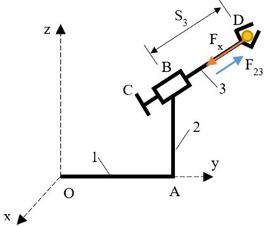
To determine the control force of member 3 (Fig. 2), the possible displacement only for generalized coordinate $q_{2}$ , where:

13

{δ q}_{1} = 0, {δ q}_{2} \neq 0, {δ φ}_{2} = 0, {δ S}_{3} \neq 0 .

The expression for total work of motion forces for this displacement, from which can be determine the generalized force $Q_{2}$ is:

14

\sum δ A_{2} = {- Q}_{2} {δ S}_{3} = F_{x} {δ S}_{3} - F_{23} {δ S}_{3}, {- Q}_{2} = \frac{\sum δ A_{2}}{{δ S}_{3}} = F_{x} - F_{23} .

Equalizing with the Lagrange’s equation for member 3, the control force is obtained as:

15

b {\ddot{S}}_{3} = {- F}_{x} + F_{23}, F_{23} = b {\ddot{S}}_{3} + F_{x} = m_{3} (- 48 t) + 2,

for:

t = 0.5 s, F_{23} = 0.546 (- 24) + 2 = - 11.104 N .

Fig. 2Determination of force F23

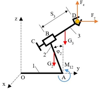
To determine the control moment of member 2, from possible displacement only for the generalized coordinate $q_{1}$ , where:

16

{δ q}_{1} \neq 0, {δ q}_{2} = 0, {δ φ}_{2} \neq 0, {δ S}_{3} = 0 .

The expression for total work of the motion forces for this possible displacement, from which can be determine generalized force $Q_{1}$ is:

17

\sum δ A_{1} = Q_{1} {δ φ}_{2} = {(G}_{2} ∙ 0.5 + G_{3} - F_{z}) l_{2} s i n φ_{2} {δ φ}_{2} - F_{y} l_{2} c o s φ_{2} {δ φ}_{2} + M_{12} {δ φ}_{2},

Q_{2} = \frac{\sum δ A_{2}}{{δ S}_{3}} = {(G}_{2} ∙ 0.5 + G_{3} - F_{z}) l_{2} s i n φ_{2} - F_{y} l_{2} c o s φ_{2} + M_{12} .

By leveling with the Lagrange's equation for member 2, the control moment is obtained as:

18

{\ddot{φ}}_{2} = {(G}_{2} ∙ 0.5 + G_{3} - F_{z}) l_{2} s i n φ_{2} - F_{y} l_{2} c o s φ_{2} + M_{12},

M_{12} = (\frac{m_{2}}{3} + m_{3}) {\ddot{φ}}_{2} - {(G}_{2} ∙ 0.5 + G_{3} - F_{z}) l_{2} s i n φ_{2} + F_{y} l_{2} c o s φ_{2} .

for:

t = 0.5 s, M_{12} = 0 - 0.324 + 1.47 = 1.146 N m .

Fig. 3Determination of moment M12

4. Design of simulation model of three-member manipulator in Matlab-Simulink

Analysis of three-member manipulator is based on a simulation model of the robot manipulator in Simulink and the obtained results will be compared with a mathematical calculation. First, laws of motion of the characteristic points from the geometry of the manipulator are written, and value of time is $t =$ 0.5 s. Manipulator kinematical and kinetostatic analysis requires to configure two joint blocks, Revolute and Prismatic. Through these two blocks the laws of motion are given $φ_{2}$ and $S_{3}$ .

Fig. 4 shows the configuration of the Joint Blot Revolute, which refers to the kinematic joint A. By increase the number of sensors/actuators to 1, so that can be define the law of motion with Joint Actuator $φ_{2}$ . The same procedure is repeat for the Prismatic Joint blocks and Fig. 5 which refers to the kinematic joint B. By increase the number of sensors/actuators to 1 so that can be define the low of motion with the Joint actuator $S_{3}$ . Using the Simulink blocks, the lows of motion are apply $φ_{2}$ and $S_{3}$ which are in function of time t, and by time differentiation angular velocity ${\dot{φ}}_{2}$ and angular acceleration ${\ddot{φ}}_{2}$ , as well as velocity ${\dot{S}}_{3}$ and acceleration ${\ddot{S}}_{3}$ , are obtained respectively. Fig. 6 shows blocks connections, signal from Clock block is connected with laws of motion $φ_{2}$ and $S_{3}$ and outputs are connected to the corresponding Joint Actuators, which are connected accordingly to the actuated Revolute and Prismatic Joint blocks.

Fig. 4Low of motion φ2

Fig. 5Low of motion S3

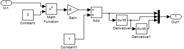
Fig. 6Block connections

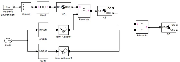
Fig. 7Manipulator simulation model

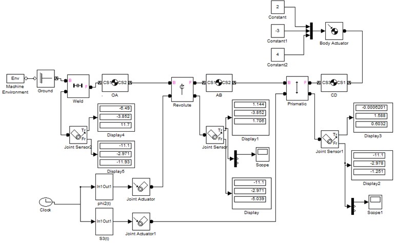
To solve the kinetostatics and to determine the control moments and forces in already created kinematic model with given control equations, first through the Body Actuator block the external forces in gripper D are applied. Additionally, in all kinematic pairs, in associated joint blocks another sensor port is added on which is connect sensors to measure the forces and moments in kinematic joints.

Projections of forces and moments in the joints can be obtained by connecting Joint sensor blocks associate already to configured Weld, Revolute and Prismatic blocks, i.e., allowing to measure the motion force and moment. Two outputs of the sensors are connected to displays showing the projections along the coordinate axes of motion force and moment. In addition, two scopes are added on which can be monitored the changes of control moment and force as function on time. This completes all settings for kinetostatic analysis of the manipulator. After simulating the model, the variations of forces and moments projections along the axes in manipulator joints at $t =$ 0.5 s can be displays.

Fig. 7 shows the complete model simulation and moments and forces in kinematic joints can be analyzed. Greater precision in Solver parameters, by select fixed-step time and in sample time can be obtained by enter a value of 0.0001.

In Simulation stop time, by entering value $t =$ 0.5 s and repeat the simulation, from Fig. 8(a) can be read the values for control force $F_{23}$ , and control moment $M_{12}$ from Fig. 8(b) which are determinate that are same as presented analytical calculations.

Fig. 8a) Control force F23, b) control moment M12

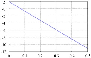
a)

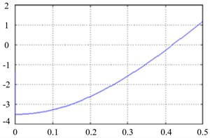
b)

5. Conclusions

Dynamic model analysis of three-member manipulator as mechanical structure is presented. The simulation of the model provides determination of motion moment $M_{12}$ in the revolute kinematic joint and motion force $F_{23}$ in prismatic kinematic joint. Mathematical analysis was performed at time $t =$ 0.5 s of force and moment by using the Lagrangian second-order equation and the principle of virtual work. The values for moments $M_{12}$ and force $F_{23}$ obtained by the analytical calculation and the values obtained by the simulation of presented dynamic model are the same. As following, this method can also be used for more complex mechanical structures for which it is difficult to analyse their dynamics, due to the fact that formation of equations of motion and solving them increase, especially if it accounts multiple points.

From presented simulation model, motion forces and moments can be determinate and through the diagrams can be analysed their values in all the kinematic joints taking in account external forces and moments as essential for designing and modelling of kinematic joints and also for control systems design.

References

Gouasmi M., Ouali M., Fernini B., Meghatria M. Kinematic modelling and simulation of a 2-R robot using solidworks and verification by MATLAB/Simulink. International Journal of Advanced Robotic Systems, Vol. 9, Issue 6, 2012, https://doi.org/10.5772/50203.

Publisher
Damic V., Cohodar M., Tvrtkovic M. Inverse dynamic analysis of hobby robot uArm by Matlab/Simulink. Annals of DAAAM and Proceedings, Vol. 27, 2016, p. 95-101.

Publisher
Arun Dayal U., Rajeevlochana C. G., Subir Kumar S. Dynamic simulation of a KUKA KR5 industrial robot using MATLAB SimMechanics. 15th National Conference on Machines and Mechanisms, 2011.

Search CrossRef
Pratap D., Mohan Reddy Y. V. Kineto-elasto dynamic analysis of robot manipulator Puma-560. IOSR Journal of Mechanical and Civil Engineering (IOSR-JMCE), Vol. 8, Issue 3, 2013, p. 33-40.

Publisher
Frankovský P., Hroncová D., Delyová I., Hudák P. Inverse and forward dynamic analysis of two link manipulator. Procedia Engineering, Vol. 48, 2012, p. 158-163.

Publisher
Atef A. A., Waleed F. F., Sa’adeh M. Y. Dynamic analysis of a two-link flexible manipulator subject to different sets of conditions. International Symposium on Robotics and Intelligent Sensors, 2012.

Search CrossRef
Shah J., Rattan S. S., Nakra B. C. Dynamic analysis of two link robot manipulator for control design using computed torque control. International Journal of Research in Computer Applications and Robotics, Vol. 3, Issue 1, 2015, p. 52-59.

Search CrossRef
Velarde-Sanchez J. A., Rodriguez-Gutierrez S. A., Garcia-Valdovinos L. G., Pedraza-Ortega J. C. 5DOF manipulator simulation based on MATLAB-Simulink methodology. 20th International Conference on Electronics Communications and Computers, Cholula, 2010, p. 295-300.

Search CrossRef
Zhao Y., Wang H. Kinematics simulation analysis and trajectory planning of a moving robot based on ADAMS. Mathematical Models in Engineering, Vol. 31, Issues 3-2, 2017, p. 71-77.

Publisher

About this article

Received

15 October 2018

Accepted

06 November 2018

Published

31 December 2018

DOI

https://doi.org/10.21595/mme.2018.20319

Keywords

manipulator

model dynamic analysis

robot model simulation

This is an open access article distributed under the Creative Commons Attribution License, which permits unrestricted use, distribution, and reproduction in any medium, provided the original work is properly cited.

Next article in issue Next

Research article

2023 01 30

Dynamic obstacle avoidance and trajectory planning of five-axis redundant industrial manipulator

Jian Ma

Research article

2022 11 26

Dynamic and vibration characteristics of flexible robot manipulator under complex electromechanical coupling

Wenhui Zhang, Zhi Wen, Yangfan Ye, Jinmiao Shen, Xiaoping Ye

Research article

2020 04 02

Experimental study on dynamic performance of pneumatic flexible manipulator with single degree of freedom

Hongbo Liu, Junye Li

Research article

2015 11 15

Coupling vibration characteristics of a translating flexible robot manipulator with harmonic driving motions

Yufei Liu, Wei Li, Yuqiao Wang, Xuefeng Yang, En Lu

H. Mickoski, I. Mickoski, and M. Djidrov, “Dynamic modeling and simulation of three-member robot manipulator,” Mathematical Models in Engineering, Vol. 4, No. 4, pp. 183–190, Dec. 2018, https://doi.org/10.21595/mme.2018.20319

Copy Extrica

Copied to clipboard!

TY  - JOUR
DO  - 10.21595/mme.2018.20319
UR  - https://doi.org/10.21595/mme.2018.20319
TI  - Dynamic modeling and simulation of three-member robot manipulator
T2  - Mathematical Models in Engineering
AU  - Mickoski, Ivan
AU  - Mickoski, Hristijan
AU  - Djidrov, Marjan
PY  - 2018
DA  - 2018/12/31
PB  - JVE International Ltd.
SP  - 183-190
IS  - 4
VL  - 4
SN  - 2351-5279
SN  - 2424-4627
ER  - 

Copy Ris

Copied to clipboard!

@article{Mickoski_2018,
	doi = {10.21595/mme.2018.20319},
	url = {https://doi.org/10.21595/mme.2018.20319},
	year = 2018,
	month = {dec},
	publisher = {{JVE} International Ltd.},
	volume = {4},
	number = {4},
	pages = {183--190},
	author = {Ivan Mickoski and Hristijan Mickoski and Marjan Djidrov},
	title = {Dynamic modeling and simulation of three-member robot manipulator},
	journal = {Mathematical Models in Engineering}
}

Copy Bibtex

Copied to clipboard!

[1]I. Mickoski, H. Mickoski, and M. Djidrov, “Dynamic modeling and simulation of three-member robot manipulator,” Mathematical Models in Engineering, vol. 4, no. 4, pp. 183–190, Dec. 2018, doi: 10.21595/mme.2018.20319.

Copy IEEE

Copied to clipboard!

Mickoski, Ivan, Hristijan Mickoski, and Marjan Djidrov. “Dynamic Modeling and Simulation of Three-Member Robot Manipulator.” Mathematical Models in Engineering 4, no. 4 (December 31, 2018): 183–90. https://doi.org/10.21595/mme.2018.20319.

Copy Chicago

Copied to clipboard!

Dynamic modeling and simulation of three-member robot manipulator

Abstract

1. Introduction

2. Manipulator characteristics

3. Manipulator kinetostatic analysis by Lagrange’s equation and principle of virtual work

4. Design of simulation model of three-member manipulator in Matlab-Simulink

5. Conclusions

References

About this article

Related Articles