Abstract
In order to reveal synchronization characteristics of a weakly damped system with two rotors mounted on different vibrating bodies, we propose a simplified physical model. Vibration of the system is discussed by the average method, which can separate fast motions (high frequency) from slow motions (low frequency). Theoretical research shows that vibration torque is the key factor to balance the energy distribution between rotors. For the system with rotational frequencies larger than the nature frequencies, the coupling characteristic frequency or characteristic frequency curve should be considered. As the coupling frequency is close to the characteristic frequency, or the vibration state is close to the characteristic frequency curve, self-synchronization of two rotors can be obtained easily.
1. Introduction
The so-called self-synchronization phenomenon corresponds to the consistency or certain relationship of systems’ parameters caused by their internal couplings and has been widely involved in non-linear vibration, hydraulic [1-3], electromechanical coupling, automatic control theory and other fields [4-8].
Huygens was the first person who observed the synchronization of pendulum clocks in the 17th Century. In [4, 5], Czolczynski et al. presented different synchronous behaves of two or pendula installed on a frame. The self-synchronization theory of rotors was developed by Bleckman [1, 2] with averaging method in the middle of the 20th century. Wen and Zhao et al. [7] modified the averaging method and proposed the average method with two small parameters. Zhang [8] deduced the synchronization condition and the synchronization stability for the vibrating system with three rotors. Hou and Fang [9, 10] investigated a vibrating screen based on the model of a rotor-pendulum system.
The above researches are mostly focused on the synchronization of pendula or rotors installed on the same vibrating frame. In this paper, we propose a vibrating system with two rotors mounted on two different vibrating bodies.
2. Dynamical equations of the vibrating system
As shown in Fig. 1, two rotors are mounted on different vibrating bodies. The vibrating body () ( 1, 2) can move in horizontal direction () and is installed on the foundation by the spring. The two bodies are connected by a coupling spring. Counterclockwise direction is taken as positive. Inertia moment and eccentricity of the rotor on its mass center are given by and . Other variables are show in Fig. 1. In this paper, synchronization of rotors is analyzed in a non-resonant vibrating system, in which rotation frequencies of rotors are larger than nature frequencies of vibrating bodies. The system is denoted as after-resonance system. We assume that , , , where , .
Fig. 1Simplified model of the system
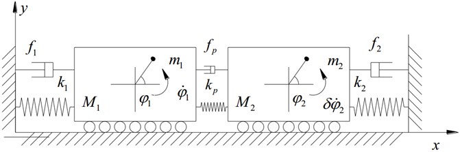
The electromagnetic torque and resistance moment of the driving motor are and () respectively. When ( 1, 2) fluctuates near the frequency , the influence of electromagnetic leakage can be neglected, and the driving force of induction motor can be linearized as , where , , , and (1, 2) correspond to the pole number, mutual inductance, synchronous speed, stator inductance and rotor resistance of the motor; is the voltage amplitude. As self-synchronization of rotors is achieved, speed fluctuations of rotors are small [1, 2]. Therefore, small variables can be neglected. Introducing , , and , we have:
The synchronous speed of two rotors is denoted by . When self-synchronization of rotors is achieved [1, 3], phases of the two rotors can be denoted as , , where and are slowly-varying parameters. From Eq. (1), we obtain:
where:
, , and show the coupling effects in the system. Rotors are driven by motors, and the resistance is approximately proportional to its speed. The average values of resultant torques of rotors are denoted by , . As the system is stable, we have:
where is the vibration torque (VT). Introducing the variable substitutions:
can be obtained. Thus, the synchronization condition can be expressed as follows [1]:
The stability criterion of the synchronous state can be discussed based on Lyapunov stability theory, it can be deduced as:
3. Discussions of theoretical results
In this paper, two rotors rotate in the same direction, that is, 1. In this paper, 0.14 H, 0.12 H, 0.6 , 314 rad/s, 220 V, 2 and other parameters of the system are shown in Table 1.
Table 1Parameters of the system
Parameters | [kg] | [kg] | [kg·m2] | [m] | [N·s/m] | [N/m] | [N·m·s/rad] |
Rotor 1 | 300 | 3.5 | 0.3 | 0.15 | 200 | 7.5×10⁵ | 3×10⁻² |
Rotor 2 | 200 | 2.5 | 0.3 | 0.1 | 200 | 7.4×10⁵ | 1.47×10⁻¹ |
We take into consideration. can be obtained easily. Thus, is the maximum vibration torque of the system (MVT). For the after-resonance system, denominator of may be zero when come to be a specific value . is deduced as:
is called the characteristic frequency (CF) of the system, as shown in Fig. 2(a) and Fig. 3. In the coordinates of and , the characteristic curve composed of characteristic frequencies at different synchronous speeds is shown in Fig. 2(b). The curve of accompanied with is shown in Fig. 3 when is a certain value (for example, 155 rad/s). The synchronous speed varies with the stiffness of the coupling spring and it can be obtained by numerical simulation.
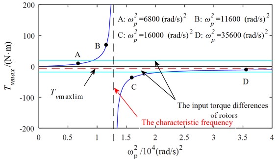
When approach from the left side, tends to infinity; when continues to increase over to infinity, gradually decreases and tends to a constant value. In Fig. 3, the curve is divided into four parts by the curves of . The four parts are denoted by LA (passing through point A), LB (passing through point B), LC (passing through point C) and LD (passing through point D) respectively. According to Eq. (4), self-synchronization of two rotors cannot be obtained when system state occurs on LA and LD; On the contrary, rotations of two rotors can be self-synchronizing when system state occurs on LB and LC.
As coupling frequency is close to the characteristic frequency , or the system state is near the characteristic frequency curve, the system coupling performance is strong, and the self synchronization of two rotors can be obtained easily. And it is convenient to control the synchronization performance by adjusting the coupling spring stiffness .
Fig. 2Surface of the maximum vibration momentvarying with the coupling frequency and synchronous speed in the after-resonance system
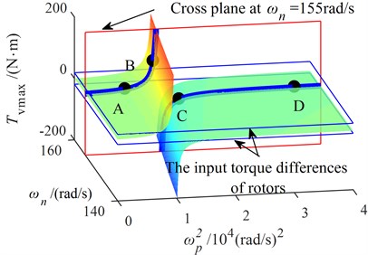
a) The three-dimensional diagram
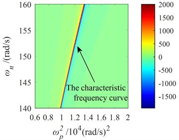
b) The two-dimensional diagram
Fig. 3Relationship between the maximum vibration moment and coupling frequency
4. Simulations for synchronization of two rotors
Simulations are carried out with set to be 6800 (rad/s)2, 11600 (rad/s)2, 16000 (rad/s)2, 35600 (rad/s)2 and infinity respectively, corresponding to points A, B, C and D.
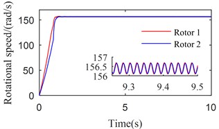
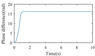
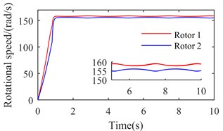
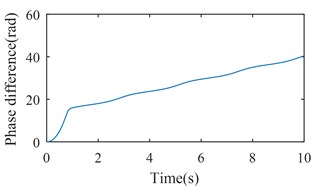
Fig. 4 shows the simulation results with 6800 (rad/s)2. From Figs. 2 and 3, we can suggest that rotations of two rotors would not be self-synchronizing in this case. As shown in Fig. 4, speeds of the two rotors are not consistent. Fig. 5 shows the simulation results with 11600 (rad/s)2. In this case, . is calculated to be 3.28 rad. As shown in Fig. 5, speeds of the two rotors reach the same value around 1.5 s, and is stable at 15.83 rad (15.83 – 4 × = 3.26 (rad)). Fig. 6 shows the simulation results with 16000 (rad/s)2. Parameters of system satisfy the self-synchronization conditions in this case too. is calculated to be 3.65 rad. As shown in Fig. 6, speeds of the two rotors reach the same value around 1.5 s, and is stable at 16.21 rad (16.21 – 4 × = 3.64 (rad)). The numerical results in Figs. 5 and 6 are consistent with the theoretical analysis.
Fig. 4Simulation results of the after-resonance system when the coupling stiffness is 1.36×10⁶ N/m
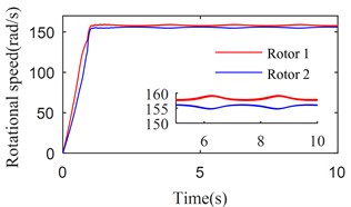
a) Rotational speeds of two rotors
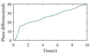
b) The phase difference between two rotors
Fig. 5Simulation results of the after-resonance system when the coupling stiffness is 2.32×10⁶ N/m
a) Rotational speeds of two rotors
b) The phase difference between two rotors
Fig. 6Simulation results of the after-resonance system when the coupling stiffness is 3.20×10⁶ N/m
a) Rotational speeds of two rotors
b) The phase difference between two rotors
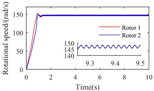
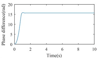
Fig. 7Simulation results of the after-resonance system when the coupling stiffness is 7.12×10⁶ N/m
a) Rotational speeds of two rotors
b) The phase difference between two rotors
Fig. 8Simulation results of the after-resonance system when the coupling stiffness is tending to infinity
a) Rotational speeds of two rotors
b) The phase difference between two rotors
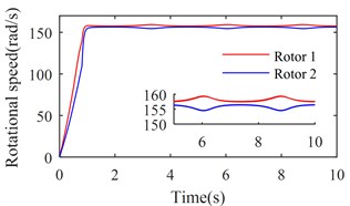
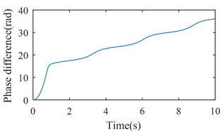
Figs. 7 and 8 show the simulation results when is set to be 35600 (rad/s)2 and tend to infinity respectively. According to Figs. 2 and 3, rotations of two rotors would not be self-synchronizing in these cases. As shown in Figs. 7(a) and 8(a), speeds of the two rotors are not consistent when the system reaches stable conditions; Figs. 7(b) and 8(b) demonstrate the asynchrony of the two rotors. Simulation results confirm the theoretical analysis.
5. Conclusions
Self-synchronization of two rotors can be observed in a weakly damped non-resonant vibrating system with two rotors mounted on different bodies. The synchronization condition is that the vibration torque is large enough to overcome the input torque difference between two rotors. For the after-resonance system, there is a characteristic frequency or characteristic frequency curve. As the coupling frequency is close to the characteristic frequency, the coupling effects of the system can be strong, and self-synchronization of two rotors occurs easily. While there is a big difference between the coupling frequency and the characteristic frequency, self-synchronization will not be achieved.
References
-
Blekhman I. I. Synchronization in Science and Technology. ASME Press, New York, USA, 1988.
-
Blekhman I. I. Vibrational Mechanics. World Scientific, Singapore, 2000.
-
Wen B. C., Fan J., Zhao C. Y., Xiong W. L. Vibratory Synchronization and Controlled Synchronization in Engineering. Science Press, Beijing, China, 2009.
-
Czolczynski K., Perlikowski P., Stefanski A., Kapitaniak T. Clustering of Huygens’ clocks. Progress of Theoretical Physics, Vol. 122, Issue 4, 2009, p. 1027-1033.
-
Czolczynski K., Perlikowski P., Stefanski A., Kapitaniak T. Why two clocks synchronize: energy balance of the synchronized clocks. Chaos, Vol. 21, Issue 2, 2011, p. 023129.
-
Wen B. C., Zhang H., Liu S. Y., He Q., Zhao C. Y. Theory and Techniques of Vibrating Machinery and Their Applications. Science Press, Beijing, China, 2010.
-
Zhao C. Y., Zhu H. T., Zhang Y. M. Synchronization of two coupled exciters in a vibrating system of spatial motion. Acta Mechanica Sinica, Vol. 26, Issue 3, 2010, p. 477-493.
-
Zhang X. L., Wen B. C., Zhao C. Y. Experimental investigation on synchronization of three co-rotating non-identical coupled exciters driven by three motors. Journal of Sound and Vibration, Vol. 333, Issue 13, 2014, p. 2898-2908.
-
Fang P., Hou Y. J., Nan Y. H., Yu L. Study of synchronization for a rotor-pendulum system with Poincare method. Journal of Vibroengineering, Vol. 17, Issue 5, 2015, p. 2681-2695.
-
Fang P., Yang Q. M., Hou Y. J., Chen Y. Theoretical Study on self-synchronization of two homodromy rotors coupled with a pendulum rod in a far-resonant vibrating system. Journal of Vibroengineering, Vol. 16, Issue 5, 2014, p. 2188-2695.
About this article

This study is supported by International Science and Technology Cooperation Program of China (Grant No. 2015DFR70660).
