Abstract
In this article, the free vibrations of Euler-Bernoulli and Timoshenko beams with arbitrary varying cross-section are investigated analytically using the perturbation technique. The governing equations are linear differential equations with variable coefficients and the Wentzel, Kramers, Brillouin approximation is adopted for solving these eigenvalue equations and determining the natural frequencies and mode shapes. This method relates the solution of equations with the solving of some successive algebraic equations. A parametric study is performed and the effects of different profiles and different combinations of boundary conditions on the natural frequencies are investigated. To confirm the reliability of the present method, the analytical results are checked with those obtained from the finite elements method and other literatures which are found to be in a good agreement. The calculations show that the presented procedure is very effective to find the modal characteristics of the varying cross-sections beams.
1. Introduction
A beam is an important element which is used as a part of some structures. To achieve a better distribution of rigidity and reducing the weight, the beams with variable cross-sections are used. The dynamic analysis of beams is frequently encountered in engineering practices. This analysis becomes more complicated in the cases of beams with the variable cross-section. The wind turbine blades are a typical example of the beams with variable thickness subjected to dynamic loads.
The natural frequency is a design parameter associated with engineering vibrations. During the past decades, the extensive research efforts have been presented concerning the linear dynamic analysis of beams. Jategaonkar and Chehil [1] determined the natural frequencies of a linear Euler-Bernoulli (E-B) beam with varying section properties by evaluating the effective inertia, area, and mass. An approximated finite elements (FE) method was introduced by Eisenberger and Reich [2] to analyze the non-uniform beams. They used the displacement functions of a constant cross-section beam to find the approximated stiffness and consistent mass matrices. Rossi and Laura [3] determined the natural frequencies and dynamic behavior of linearly tapered Timoshenko beams subjected to different combinations of edge supports by the FE procedures. De Rosa and Auciello [4] studied the dynamic behavior of beams with a linearly varying cross-section. The equation of motion was solved in terms of Bessel functions. Abrate [5] presented simple formulas for predicting the fundamental natural frequency of non-uniform beams with the general shape and arbitrary boundary conditions by Rayleigh-Ritz method. Zhou and Cheung [6] studied the vibrational characteristics of tapered E-B beams with a continuously varying rectangular cross-section by the Rayleigh-Ritz method. Byoung et al. [7] studied the free vibrations of tapered E-B beams with general boundary conditions. The natural frequencies were calculated by combining the Runge-Kutta and the determinant search methods. Kukla and Zamojska [8] applied Green’s function method for frequency analysis of an E-B beam with the varying cross-section. Rensburgand and Merweb [9] presented a systematic approach to solve the eigenvalue problems associated with the uniform Timoshenko beam model by the FE method. Ece et al. [10] studied the vibrations of an isotropic E-B beam which has a variable cross-section. The governing equation was reduced to an ordinary differential equation in spatial coordinate for a family of cross-section geometries with exponentially varying width. De Rosa and Lippiello [11] studied the natural frequencies of tapered beams by using the E-B theory in the presence of an arbitrary number of rotationally, axially and elastically flexible constraints. The dynamic analysis was performed by means of the cell discretization method. Zamorska [12] used Green’s function and power series methods for the free vibrations problem of non-uniform E-B beams. Mahmoud et al. [13] applied the differential transformation method for the free vibrations analysis of E-B beams with uniform and non-uniform cross-sections. Boiangiu et al. [14] solved the differential equations for free bending vibrations of straight E-B beams with variable cross-section using Bessel’s functions. In order to improve the analytical accuracy, Leiping et al. [15] found the stiffness matrix of Timoshenko beam element with the arbitrary section. According to the relationship between geometrical deformation and internal force, by integral of sectional curvature, the shearing strain, and axial strain, the stiffness matrix of the Timoshenko beam element was derived. Yuan et al. [16] proposed a novel method to simplify the governing equations for the free vibrations of Timoshenko beams with both geometrical non-uniformity and material inhomogeneity along the beam axis. They converted the governing equations to uncoupled forms. Each of obtained equations was in the form of Sturm–Liouville type with variable coefficients. The authors solved these equations for polynomial and exponential variations of parameters which have the exact solutions in terms of Bessel’s and hypergeometric functions. Korabathina and Koppanat [17] developed the “coupled displacement field method” for calculating the fundamental frequency of Timoshenko beam which reduces the computational efforts compared with respect to the other methods. Zhao et al. [18] introduced the Chebyshev polynomials to analyze the free vibrations of axially functionally graded E-B and Timoshenko beams with a non-uniform cross-section. Chen et al. [19] re-examined the free vibrations of rotating tapered Timoshenko beams using the technique of variational iteration. Nourifar et al [20] utilized the differential transform method for free vibrations analysis of rotating E-B beam with an exponentially varying cross-section.
The review of literatures demonstrates the FE and analytical methods to find the natural frequencies in the beams. Although the FE is straight forward but building a FE model for a beam with arbitrary varying cross section, is difficult especially when the optimization with trial and error is the final purpose. In analytical filed, the most authors used the known functions for the solution to find the eigenvalue of the system. In this text, an analytical solution based on the perturbation technique is presented for the flexural vibrations of E-B and Timoshenko beams, with variable cross-section and the natural frequencies and mode shapes are determined. We do not restrict our solution for special boundary conditions, thickness profiles or using special functions for solution. The numerical examples are presented to demonstrate the accuracy and the efficiency of the presented method. The essential features and novel aspects of the presented formulation are summarized as follows:
The cross-section has an arbitrary symmetric shape and leads to the equations with variable coefficients.
An analytical procedure is demonstrated to find the eigenvalues of one or two coupled differential equations with variable coefficient.
The formulation has a short running time without any restrictions such as the mesh pattern in FE.
It is possible to use this method for different boundary conditions.
2. Euler Bernoulli beam
Consider an isotropic, homogenous non-uniform symmetric E-B beam with the length , density and cross-sectional area .
Fig. 1Schematic of beam
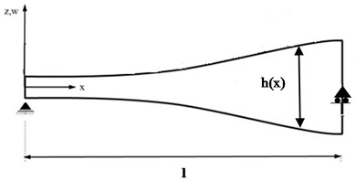
The governing equation of the beam with varying cross-section and small deflection is as [22]:
In Eq. (1), is the beam transverse displacement, , are the spatial and time parameter, is the Young modulus, , are the area moment of inertia and area cross section of the beam. The boundary conditions for E-B beam are as the following:
In this paper, the perturbation technique is used for solving the governing equations. We start by converting the governing equation to the dimensionless form, using the following parameters:
, are dimensionless location and time, respectively, is dimensionless transverse displacement, , are characteristic deflection and time, is gyration radius of the cross-section and is a small quantity which is considered as the perturbation parameter. By using Eq. (3), the dimensionless form of Eq. (1) (in terms of displacement) is as the following:
Eq. (4) is a linear partial differential equation with variable coefficients. We consider as a large parameters and use the Wentzel, Kramers, Brillouin )WKB( approximation [21] for determining the natural frequencies and mode shapes. We assume the solutions in the following form:
where is non-dimensional natural frequency. By substituting Eq. (5) into Eq. (4) we have:
We seek an expansion for in the following form:
By substituting Eq. (7) into Eq. (6) and considering a straightforward expansion for in the following form, we have:
We substitute Eqs. (7), (8) into Eq. (6), and separate different orders of as the following:
From Eq. (9), four roots for are determined. Then , can obtain From Eqs. (10), (11), so we have . The solutions of Eq. (7) is in the following form:
By applying the boundary conditions into Eqs. (12), a system of homogenous algebraic equations is constructed. The non-trivial solution of this system results eigenvalues and mode shapes.
3. Timoshenko beam
We consider the free vibrations of homogeneous Timoshenko beam with variable cross- section as follows [22]:
where denotes the rotation angle due to bending, is the shear modulus, /, and is called the Timoshenko shear correction factor, depends on the geometry. The shear correction is introduced to take care of the non-uniformity in the shear force across the section. For a rectangular section 1.20, for a circular section 1.11 [22]. The boundary conditions for Timoshenko beam are as follows:
Combining two equations gives a forth order differential equation with variable coefficient as follows:
To convert the equation as dimensionless we use Eqs. (3). Substitution Eqs (3) into Eq. (15) gives a dimensionless equation of motion represented by:
We seek an expansion for in Eq. (16) in the following form:
Substituting Eq. (17) into Eq. (16) and applying a straightforward expansion for as Eq. (8) and, separating the terms with the same order of results:
From Eq. (18) four roots for are determined, subsequently substituting Eq. (19), (20) gives , so we have and the solutions is in the following form:
By applying Eq. (5) into the first Eqs. (13), and using Eq. (3) to convert the resultant equation to dimensionless form and substituting Eq. (21) in the obtained equation, it is possible to calculate the transverse displacement . Consequently, is determined from Eq. (5). By applying, the boundary conditions (Eqs. 14), a system of homogenous algebraic equations is constructed. For a non-trivial solution, the coefficient matrix has to equate to zero. The solutions of this equation which are determined by the bisection method are the natural frequencies of the system.
4. FE analysis
ANSYS Workbench 16.2 FE package has been used for the modal analysis of the variable section beam. All the reported results (except that mentioned cases) are related to the rectangular cross-section with constant width and variable thickness with the characteristics listed in Table 1.
Table 1Beam properties
Length (mm) | 500 |
Width (mm) | 32 |
(mm) | 25 |
(mm) | 45 |
Elastic modulus (GPa) | 200 |
(kg/m3) | 7800 |
, are the section diameter and thickness of the circular and rectangular cross-sections at 0 respectively and , related to 1 | |
5. Parametric study
The analytical calculations have been performed on Maple mathematical environment. As case studies, we consider the beams with rectangular cross section and constant, linear, parabolic, trigonometric thickness distributions. All the reported frequencies are dimensionless and by multiplying in (Eq. (3)), one can find them in terms of rad/s. To check the formulation, we investigate at first the beam with constant and linear thicknesses variations. Table 2 shows the frequencies of the E-B and Timoshenko beams with constant thicknesses and simply supported (SS) boundary conditions. The results have been reported for two cases: E-B(HG) and Timoshenko (HG) which are related to the exact solution of equations [22] and WKB which is for the presented formulation. It is seen that the difference between the results is small, so the program works correctly. Also, for the higher modes, the difference between the approximated and exact methods increases. From Table 2, by decreasing the ration of the length to thickness (), the natural frequencies and the difference between E-B and Timoshenko theories increase especially in the higher modes. The difference percentage of results for HG has been defined as:
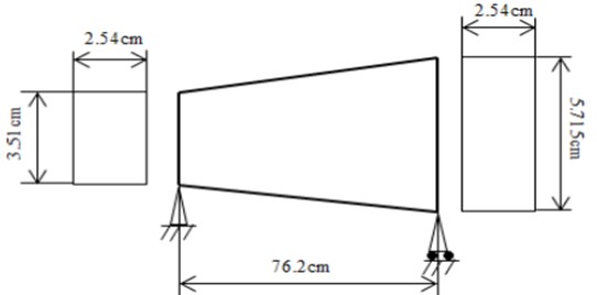
In Table 3, a comparison of E-B and Timoshenko beams with the results of Shukla [23] has been reported for the linear thickness profile (Fig. 2) and simply supported boundary conditions. Shukla [23] used the E-B theory and the FE method for determining the natural frequencies. The results show that in the higher modes, the Timoshenko results are closer to the FE solution with respect to the E-B.
Table 2Comparison of E-B and Timoshenko beams with constant thickness (SS)
Theory | 1st mode | 2nd mode | 3rd mode | |
25 | E-B (HG) | 0.11397 | 0.45584 | 1.02570 |
E-B (WKB) | 0.11396 | 0.45586 | 1.02568 | |
Timoshenko (HG) | 0.11368 | 0.45131 | 1.00307 | |
Timoshenko (WKB) | 0.11396 | 0.45588 | 1.02590 | |
Diff (%) | 0.25 | 1.00 | 2.26 | |
15.6 | E-B(HG) | 0.18262 | 0.73053 | 1.64365 |
E-B(WKB) | 0.18264 | 0.73054 | 1.64372 | |
Timoshenko (HG) | 0.18146 | 0.71225 | 1.55617 | |
Timoshenko (WKB) | 0.18264 | 0.73075 | 1.64610 | |
Diff (%) | 0.64 | 2.57 | 5.62 | |
10 | E-B (HG) | 0.28489 | 1.13969 | 2.56422 |
E-B (WKB) | 0.28491 | 1.13964 | 2.56420 | |
Timoshenko (HG) | 0.28048 | 1.07442 | 2.02705 | |
Timoshenko (WKB) | 0.28494 | 1.14158 | 2.58680 | |
Diff (%) | 1.57 | 6.07 | 26.50 |
Table 3Comparison of E-B and Timoshenko beams with results of Shukla (2013)
Theory | 1st mode | 2nd mode | 3rd mode |
Shukla (2013) | 0.17145 | 0.70560 | 1.58791 |
E-B | 0.19390 | 0.78484 | 1.76270 |
Diff (%) | 1.35 | 3.33 | 3.47 |
Timoshenko | 0.17400 | 0.68034 | 1.52548 |
Diff (%) | 1.49 | 3.58 | 3.93 |
Fig. 2Simply supported beam with linearly variable thickness (E= 2.109 GPa, ρ= 7995.74 Kg/m3) (Shukla, 2013)
The various functions with equal volume for the beam area cross section constant) has been considered. For the rectangular cross section, and the various thickness functions has been listed in Table 4 and comparison of the frequencies of E-B and Timoshenko beam have been reported in Table 5. The differences percentage has been defined similar Table 2.
Table 4Thickness profile with different functions
Type 1 | 0.8, 1 | |
Type 2 | –1.6, , 1 | |
Type 3 | –1, , 1 | |
Type 4 | –0.4, 1.4 | |
Type 5 | 0.866, , 1.4 |
Table 5Comparison of E-B and Timoshenko beams with different thickness functions (SS)
Thickness function | Theory | 1st mode | 2nd mode | 3rd mode |
Type 1 | E-B | 0.19390 | 0.78484 | 1.76270 |
Timoshenko | 0.19367 | 0.78517 | 1.76637 | |
Diff (%) | 0.12 | 0.04 | 0.21 | |
Type 2 | E-B | 0.20686 | 0.78304 | 1.74937 |
Timoshenko | 0.20218 | 0.78190 | 1.75233 | |
Diff (%) | 2.32 | 0.15 | 0.17 | |
Type 3 | E-B | 0.23235 | 0.79136 | 1.75057 |
Timoshenko | 0.18676 | 0.77510 | 1.74662 | |
FE | 0.18606 | 0.75727 | 1.63868 | |
Diff (%) | 24.41 | 2.10 | 0.23 | |
Type 4 | E-B | 0.20195 | 0.78161 | 1.74759 |
Timoshenko | 0.20198 | 0.78201 | 1.75122 | |
Diff (%) | 0.02 | 0.05 | 0.21 | |
Type 5 | E-B | 0.19337 | 0.78493 | 1.76358 |
Timoshenko | 0.19343 | 0.78528 | 1.76726 | |
Diff (%) | 0.03 | 0.04 | 0.21 |
According to Table 5, the different profiles with the same weight can change the frequencies or distribution of density is important. For profile Type 3, there is a discrepancy between Timoshenko and E-B frequencies. For more investigation, we analyzed this case using the FE procedure. It is seen the obtained results for the FE and Timoshenko are nearly the same, but the E-B result is not confidence.
Tables 6 and 7 comprise three first frequencies of E-B and Timoshenko beams with thickness variation (Type 2) for some different boundary conditions. The notations C and S stand for the clamped and simply supported boundary conditions respectively. In SC, SS, CC, … the former letter indicates boundary condition at 0 and the latter one indicates the boundary condition at 1 e.g. SC stands for the simply supported at 0 and clamped at 1. Tables 6 demonstrate that the highest frequency corresponds to the CC boundary conditions while the lowest frequency occurs for SS which was expected. Also the results for two ( (2)), and three terms ( (3)) in the expansion have been reported in these tables. Although the differences of results in the most cases are small but for the non-similar boundaries (i.e. SC, CS) in E-B theory, the obtained results from two terms expansion are in doubt because it reports the same frequencies for the SC and CS. So, we reported the results for three terms expansion.
Table 6E-B and Timoshenko results with two and three terms (Type 2)
– | Mode | SS (2) | SS (3) | Diff (%) | CC (2) | CC (3) | Diff (%) |
E-B | 1 | 0.19337 | 0.20686 | 6.52 | 0.43835 | 0.44665 | 1.86 |
2 | 0.77349 | 0.78304 | 1.22 | 1.20833 | 1.21696 | 0.71 | |
3 | 1.74035 | 1.74937 | 0.52 | 2.36882 | 2.37744 | 0.36 | |
Timoshenko | 1 | 0.19360 | 0.20218 | 4.24 | 0.43984 | 0.44824 | 1.87 |
2 | 0.77265 | 0.78190 | 1.18 | 1.21641 | 1.22533 | 0.73 | |
3 | 1.74317 | 1.75233 | 0.52 | 2.39684 | 2.40613 | 0.39 |
Table 7E-B and Timoshenko results with two and three terms (Type 2)
– | Mode | CS (2) | CS (3) | Diff (%) | SC (2) | SC (3) | Diff (%) |
E-B | 1 | 0.30208 | 0.28920 | 4.26 | 0.30208 | 0.33338 | 9.39 |
2 | 0.97894 | 0.97321 | 0.59 | 0.97894 | 1.00235 | 2.34 | |
3 | 2.04249 | 2.04058 | 0.09 | 2.04249 | 2.06190 | 0.94 | |
Timoshenko | 1 | 0.23490 | 0.27123 | 13.4 | 0.34988 | 0.34404 | 1.70 |
2 | 0.95222 | 0.97010 | 1.84 | 1.00968 | 1.01050 | 0.08 | |
3 | 2.03441 | 2.04911 | 0.72 | 2.07621 | 2.08000 | 0.18 |
In Table 8 comparison of three first frequency of E-B and Timoshenko beams with various cross-sections, SS boundary conditions and the thickness variation Type 2 have been listed. The beam with different sections and the same volume have different frequencies. Also, the Timoshenko theory does not have advantage with respect to the E-B for calculating the first frequency of the beam with the circular section in this case study.
Table 8Comparison of E-B and Timoshenko beams with various cross-sections profile (Type 2-SS)
Beam section | Theory | 1st mode | 2nd mode | 3rd mode |
Rectangular | E-B | 0.20686 | 0.78304 | 1.74937 |
Timoshenko | 0.20218 | 0.78190 | 1.75233 | |
Circular | E-B | 0.35916 | 1.33839 | 2.97013 |
Timoshenko | 0.32000 | 0.96993 | 2.14803 | |
– | FE | 0.38061 | 1.04338 | 1.97235 |
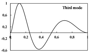
In Fig. 3 three first mode shapes of the E-B beam with CC conditions have been shown. In despite of the beams with constant thickness, for a beam with variable thickness the intersection point of mode shape curve with the horizontal axis is not exactly in the middle of the beam.
Fig. 3Three mode shapes for thickness E-B beam (Type 2, CC)
a)
b)
c)
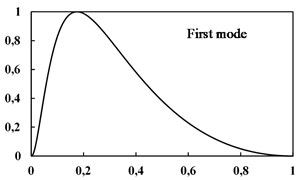
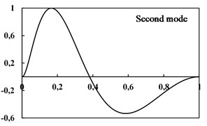
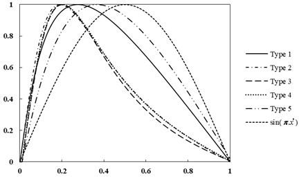
In Fig. 4 the effect of thickness function on the first mode shape of the E-B beam with SS boundary conditions can be seen. As shown, the sinusoidal function is not suitable for the mode shape in beams with variable thickness and the peak of the graph is not necessarily at the mid-point of the non-uniform beam.
Fig. 4First mode shape for five type’s thickness functions of E-B beam (SS)
6. Conclusions
A mathematical approach has been applied to investigate the free vibration of E-B and Timoshenko beams with arbitrary symmetric variable cross-section. The governing equations were solved analytically by the perturbation technique. A sensitivity analysis was performed to investigate the influences of boundary conditions, cross-section shape and various thickness functions on the transverse natural frequency of the beam. In summary:
1) An arbitrary cross-section led to differential motion equation with variable coefficients. Using WKB approximation, new form of equations can obtain which, has a closed-form solution in each order of .
2) The calculations can be performed using a simple code in a mathematical environment such as Maple and it is not necessary to construct a FE model. In the other word, the calculations can be performed faster than the FE and this study provides a unified and systematic procedure which is seemingly simpler and more straightforward than the other methods.
3) By using the proposed method, any natural frequency and mode shape function can be obtained one at a time.
4) The presented method can use for different boundary conditions.
5) By increasing the thickness, the natural frequency increases and the difference between E-B beam and Timoshenko beam increases.
6) The boundary conditions have less effect for higher modes.
7) It can be seen that the variation of cross-section has a significant effect on the mode shapes. The known trial functions that satisfy the geometric boundary conditions such as sinusoidal function are not suitable as admissible functions for mode shapes in a beam with variable thickness in the methods such as Galerking.
8) It is also possible to use this method for the other cross-section shapes and it can also be useful for designing non-uniform E-B and Timoshenko beams which may be required to vibrate with a particular frequency.
References
-
Jategaonkar R., Chehil D. S. Natural frequencies of a beam with varying section properties. Journal of Sound and Vibration, Vol. 133, 1989, p. 303-322.
-
Eisenberger M., Reich Y. Static, vibration and stability analysis of non-uniform beams. Journal of Computers and Structures, Vol. 31, Issue 4, 1989, p. 567-573.
-
Rossi R. E., Laura P. A. A. Numerical experiments on vibrating, linearly tapered Timoshenko beams. Journal of Sound and Vibration, Vol. 168, 1993, p. 179-183.
-
De Rosa M. A., Auciello N. M. Free vibrations of tapered beams with flexible ends. Journal of Computers and Structures, Vol. 60, Issue 2, 1996, p. 197-202.
-
Abrate S. Vibration of non-uniform rods and beams. Journal of Sound and Vibration, Vol. 185, Issue 4, 1995, p. 703-716.
-
Zhou D., Cheung Y. K. The free vibration of a type of tapered beams. Journal of Computer Methods in Applied Mechanics and Engineering, Vol. 188, 2000, p. 203-216.
-
Byoung K. L., Jong K. L., Tae E. L., Sun G. K. Free vibrations of tapered Beams with general boundary condition. Journal of Civil Engineering, Vol. 6, Issue 3, 2002, p. 283-288.
-
Kukla S., Zamojska I. Application of Green’s function method in free vibration analysis of non-uniform beams. Scientific Research of the Institute of Mathematics and Computer Science, Vol. 4, Issue 1, 2005, p. 87-94.
-
Rensburga N. F. J. V., Merweb A. J. V. D. Natural frequencies and modes of a Timoshenko beam. Wave Motion, Vol. 44, 2006, p. 58-69.
-
Ece M. C., Aydogdu M., Taskin V. Vibration of a variable cross-section beam. Journal of Mechanics Research Communications, Vol. 34, 2007, p. 78-84.
-
De Rosa M. A., Lippiello M. Natural vibration frequencies of tapered beams. Journal of Engineering Transactions, Vol. 57, Issue 1, 2009, p. 45-66.
-
Zamorska I. Free transverse vibrations of non-uniform beams. Scientific Research of the Institute of Mathematics and Computer Science, Vol. 9, Issue 2, 2010, p. 244-250.
-
Mahmoud A. A., Abdelghany S. M., Ewis K. M. Free vibrations of uniform and non-uniform E-B beam using differential transformation method. Asian Journal of Mathematics and Applications, 2013.
-
Boiangiu M., Ceasus V., Untaroiu C. D. A transfer matrix method for free vibration analysis of Euler-Bernoulli beams with variable cross-section. Journal of Vibration and Control, Vol. 22, Issue 11, 2014, p. 2591-2602.
-
Leiping X., Pengfei H., Bing H. Stiffness matrix of Timoshenko beam element with arbitrary variable section. 6th International Conference on Machinery, Materials, Environment, Biotechnology and Computer, 2016.
-
Yuan J., Pao Y. H., Chen W. Exact solutions for free vibrations of axially inhomogeneous Timoshenko beams with variable cross-section. Acta Mechanica, Vol. 227, 2016, p. 2625-2643.
-
Korabathina R., Koppanat M. S. Linear free vibration analysis of tapered Timoshenko beams using coupled displacement field Method. Journal of Mathematical Models in Engineering, Vol. 2, Issue 1, 2016, p. 27-33.
-
Zhao Y., Huang Y., Guo M. A novel approach for free vibration of axially functionally graded beams with non-uniform cross-section based on Chebyshev polynomials theory. Journal of Composite Structure, Vol. 168, 2017, p. 277-284.
-
Chen Y., Zhang J., Zhang H. Free vibration analysis of rotating tapered Timoshenko beams via variational iteration method. Journal of Vibration and Control, Vol. 23, Issue 2, 2017, p. 220-234.
-
Nourifar M., Keyhani A., Aftabi S. A. Free vibration analysis of rotating Euler-Bernoulli beam with exponentially varying cross-section by differential transform method. International Journal of Structural Stability and Dynamics, Vol. 18, Issue 2, 2017, p. 1850024.
-
Nayfeh A. H. Introduction to Perturbation Techniques. John Wiley, USA, 1993.
-
Hagedorn P., Gupta A. D. Vibrations and Waves in Continuous Mechanical Systems. John Wiley and Sons, USA, 1988.
-
Shukla R. K. Vibration Analysis of Tapered Beam. Department of Mechanical Engineering National Institute of Technology, Rourkela, 2013.
About this article

