Investigation of elliptical approximation in the model of the force of dry friction

Ragulskis, K.; Bubulis, A.; Paškevičius, P.; Pauliukas, A.; Ragulskis, L.

doi:10.21595/mme.2018.20001

Mathematical Models in Engineering

Browse Journal

Submit article

Published: 30 September 2018

Check for updates

Investigation of elliptical approximation in the model of the force of dry friction

K. Ragulskis¹

A. Bubulis²

P. Paškevičius³

A. Pauliukas⁴

L. Ragulskis⁵

¹Kaunas University of Technology, K. Donelaičio Str. 73, LT-44249, Kaunas, Lithuania

²Kaunas University of Technology, Mechatronics Institute, Studentų Str. 56, LT-51424, Kaunas, Lithuania

³Company “Vaivora”, Palemono Str. 2a, LT-52191, Kaunas, Lithuania

⁴Aleksandras Stulginskis University, Studentų Str. 11, LT-53361, Akademija, Kaunas District, Lithuania

⁵Vytautas Magnus University, Vileikos Str. 8, LT-44404, Kaunas, Lithuania

Corresponding Author:

K. Ragulskis

Cite the article Download PDF

Downloads 1343

CrossRef Citations 1

Abstract

In the numerical procedures involving the force of dry friction some type of numerical approximation for this investigated phenomenon is used in the process of calculations. Elliptic approximations for the local transition region are proposed, and numerical results are presented in this paper. The smoothness and continuity of this approximation is demonstrated by several computational experiments.

1. Introduction

Engineering problems and investigations of vibrating systems using various numerical procedures involving the force of dry friction are important in practical applications. Applications of various types of numerical approximations for this phenomenon are common. In the presented investigation elliptic approximation of the local transition region is proposed. Computational experiments are performed for typical problems and numerical results are presented. This approximation has good smoothness and continuity properties. Thus, it is advantageous in various numerical procedures.

This paper is a continuation of investigations for numerical representation of the similar model for the force of dry friction presented in [1]. Piecewise linear approximations of the model for the force representing dry friction as well as numerical investigations of various nonlinear problems of vibrations of mechanical systems are presented in [2]. Essentially nonlinear dynamical systems and their analytical as well as computational investigations are presented in [3]. Basic models of vibrating systems and their investigations are presented in [4]. Contemporary methods of investigation of vibrating systems are described in [5]. Basic models of vibrating systems and their analysis are described in [6]. Vibrating dynamical systems and their contemporary applications are presented in [7].

Numerical procedures of integration of vibrating mechanical systems are presented in [8]. Related presentation of numerical procedures for integration of vibrating systems is available in [9]. Method of integration using finite elements in time is described in [10]. More detailed description of the numerical methods based on finite elements in time is available in [11]. Numerical procedures for integration of differential equations of first order are presented in [12].

Solutions of various basic problems involving the force of dry friction are given in [13].

Nonlinear effects are important in problems of surface cleaning and they are described in [14]. The process of cleaning is also investigated in [15]. Interactions of particles with surfaces are investigated in [16]. Interactions of particles with surfaces of larger particles are analysed in [17]. Measurements of adhesion of particles are described in [18]. Related experimental investigations of particles using atomic force microscopy are presented in [19]. The investigations of numerical representation of the investigated model of the force representing dry friction are important for their possible use in the models of surface cleaning.

2. Investigation of elliptic representation for the analyzed force representing dry friction

Further $u$ denotes displacement of the mechanical system, $H$ represents the approximate model for the investigated force representing dry friction, while the dot over the variable is used to denote the operation of differentiation performed with respect to the time variable $t$ .

The numerical value of the variable representing velocity at the beginning of the local transition interval between the constant values of the force representing the investigated dry friction is denoted as ${\dot{u}}_{1}$ and the numerical value of the variable representing velocity at the end of the local transition interval between the constant values of the force representing the investigated dry friction is denoted as ${\dot{u}}_{2}$ . The average value is calculated as:

1

{\dot{u}}_{c} = \frac{{\dot{u}}_{1} + {\dot{u}}_{2}}{2} .

The value of the approximation for the force representing dry friction at the beginning of the local transition interval interconnecting the constant values for the force representing dry friction is denoted as $H_{1}$ and the value of the force representing dry friction at the end of the local transition interval interconnecting the constant values for the force representing dry friction is denoted as $H_{2} .$ The average value is calculated as:

2

H_{c} = \frac{H_{1} + H_{2}}{2} .

The following quantities denoting one half of the difference of the previously defined values are introduced:

3

a = \frac{H_{2} - H_{1}}{2},

4

b = \frac{{\dot{u}}_{2} - {\dot{u}}_{1}}{2} .

The approximation of the transition region is based on the following elliptical equations:

5

\frac{{(H - H_{c})}^{2}}{a^{2}} + \frac{{(\dot{u} - ({\dot{u}}_{c} - b))}^{2}}{b^{2}} = 1,

6

\frac{{(H - H_{c})}^{2}}{a^{2}} + \frac{{(\dot{u} - ({\dot{u}}_{c} + b))}^{2}}{b^{2}} = 1 .

The following elliptic function is introduced:

7

E ({\dot{u}}_{1}, {\dot{u}}_{2}, H_{1}, H_{2}, \dot{u}) = \{\begin{array}{l} H_{c} - a \sqrt{1 - {(\frac{\dot{u} - ({\dot{u}}_{c} - b)}{b})}^{2}}, \dot{u} \leq {\dot{u}}_{c}, \\ H_{c} + a \sqrt{1 - {(\frac{\dot{u} - ({\dot{u}}_{c} + b)}{b})}^{2}}, \dot{u} > {\dot{u}}_{c} . \end{array}

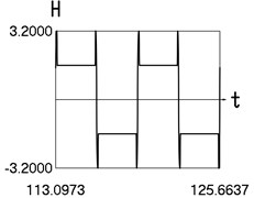
The force of dry friction is approximated as:

8

H = \{\begin{array}{l} E (- Δ, Δ, - h, h, \dot{u}), & |\dot{u}| < Δ, \\ h, & |\dot{u}| \geq Δ, \dot{u} > 0, \\ - h, & |\dot{u}| \geq Δ, \dot{u} < 0, \end{array}

where $h$ denotes the coefficient representing the dry friction, while $Δ$ represents the width of the interval for transition between the required values.

The analyzed nonlinear mechanical system is represented by the following numerical model:

9

m \ddot{u} + c \dot{u} + k u = P s i n ω t - H,

where $m$ is the notation used for the mass of the investigated system, $c$ denotes the coefficient representing the force of viscous friction, $k$ denotes the coefficient representing the stiffness of the investigated mechanical system, $P$ denotes the amplitude of the force which excites the vibrating motion, $ω$ denotes the frequency of the force performing excitation.

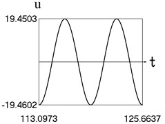
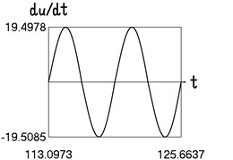
In the performed investigation values of the parameters of the analyzed nonlinear system were given the quantities: $ω =$ 1, $h =$ 3.2, $P =$ 4, $m =$ 1, $c =$ 0.1, $k =$ 1. In the numerical investigations zero initial conditions were assumed. Steady state motion was investigated. Two periods were represented.

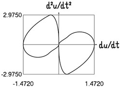
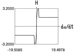
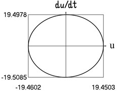
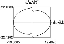
Results for $Δ =$ 0.8 are shown graphically in Fig. 1.

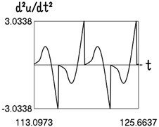
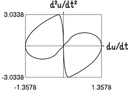
Some of the results for $Δ = 0.4$ are shown graphically in Fig. 2.

Some of the results for $Δ = 0.2$ are shown graphically in Fig. 3.

Fig. 1Motion in steady state regime for wide transition region

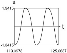
a) Time history of displacement

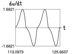
b) Time history of velocity

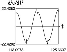
c) Time history of acceleration

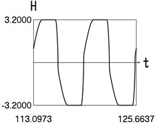
d) Time history of $H$

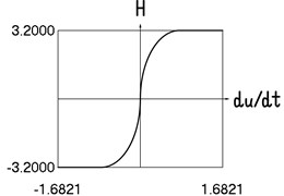
e) Dependence of $H$ from velocity

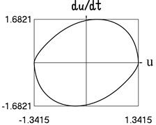
f) Dependence of velocity from displacement

g) Dependence of acceleration from velocity

The presented graphical relationships for three typical widths of the transition region show the influence of the width of the interval representing transition to the obtained numerical results. The effect of the width of the interval representing transition is especially clearly seen in the graphical relationships involving the accelerations.

Fig. 2Motion in steady state regime for transition region of medium width

a) Time history of acceleration

b) Dependence of acceleration from velocity

Fig. 3Motion in steady state regime for narrow transition region

a) Time history of acceleration

b) Dependence of acceleration from velocity

3. Investigation of more complicated model for the analyzed force representing dry friction

In this model the investigated coefficient representing dry friction increases in the vicinity of the value of velocity equal to zero. This fact is taken into account in a more complicated model of the representation for the force approximating dry friction. Here it is usually considered that it is valid $h / Δ = h_{a} / Δ_{a}$ , where $h_{a}$ denotes the increase in the approximation of the variation of the coefficient representing the force of dry friction in the investigated region, while $Δ_{a}$ defines the width of the interval representing the transition connecting the values of the investigated coefficient approximating dry friction $h$ and $h + h_{a} .$ Thus $h_{a} = h \frac{Δ_{a}}{Δ} .$

In the numerical model the force of dry friction is approximated as:

10

H = \{\begin{array}{l} E (- Δ - Δ_{a}, Δ + Δ_{a}, - h - h \frac{Δ_{a}}{Δ}, h + h \frac{Δ_{a}}{Δ}, \dot{u}), & |\dot{u}| < Δ + Δ_{a}, \\ E (Δ + Δ_{a}, Δ + 2 Δ_{a}, h + h \frac{Δ_{a}}{Δ}, h, \dot{u}), & Δ + Δ_{a} \leq |\dot{u}| < Δ + 2 Δ_{a}, \dot{u} > 0, \\ E (- Δ - 2 Δ_{a}, - Δ - Δ_{a}, - h, - h - h \frac{Δ_{a}}{Δ}, \dot{u}), & Δ + Δ_{a} \leq |\dot{u}| < Δ + 2 Δ_{a}, \dot{u} < 0, \\ h, & |\dot{u}| \geq Δ + 2 Δ_{a}, \dot{u} > 0, \\ - h, & |\dot{u}| \geq Δ + 2 Δ_{a}, \dot{u} < 0 . \end{array}

In the performed investigation values of the parameters of the analyzed nonlinear system were given the quantities: $ω =$ 1, $h =$ 1.6, $Δ =$ 0.8, $Δ_{a} =$ 0.8, $P =$ 4, $m =$ 1, $c =$ 0.1, $k =$ 1. In the numerical investigations zero initial conditions were assumed. Steady state motion was investigated. Two periods were represented.

Results of calculations are shown graphically in Fig. 4.

Typical features of dynamic behavior of the nonlinear vibrating system with more complicated model of dry friction are reproduced by this elliptic representation for approximation of the effect of dry friction.

Fig. 4Motion in steady state regime for more complicated model of the force approximating dry friction

a) Time history of displacement

b) Time history of velocity

c) Time history of acceleration

d) Time history of $H$

e) Dependence of $H$ from velocity

f) Dependence of velocity from displacement

g) Dependence of acceleration from velocity

4. Conclusions

In engineering investigations of vibrating systems various types of nonlinear behavior are to be used in numerical procedures. It is important to use numerically acceptable approximations of this behaviour. Typical often used nonlinearity is dry friction. Usually some type of approximation for this phenomenon is used. Here elliptic approximation of the local transition region is proposed. Numerical results are presented in detail. This approximation can be noted for its high smoothness and continuity. The influence of the width of the interval interconnecting the investigated values to the results obtained from calculations is shown in the obtained graphical relationships.

Numerical analysis of the mechanical model with more advanced model of the approximation for the investigated force representing dry friction has been presented. In this model the increase of the investigated coefficient representing the force approximating the effect of dry friction in the vicinity of the value of velocity equal to zero is taken into account. Typical features of dynamic behavior of the nonlinear vibrating system with more complicated model of dry friction are reproduced by this elliptic representation for the force approximating dry friction. Based on the presented numerical results the elliptic approximation is recommended for engineering calculations involving the action of force representing the effect of dry friction.

References

Ragulskis K., Paškevičius P., Bubulis A., Pauliukas A., Ragulskis L. Improved numerical approximation of dry friction phenomena. Mathematical Models in Engineering, Vol. 3, Issue 2, 2017, p. 106-111.

Publisher
Levy S., Wilkinson J. P. D. The Component Element Method in Dynamics with Application to Earthquake and Vehicle Engineering. McGraw-Hill, New York, 1976.

Search CrossRef
Ragulskienė V. Vibro-Shock Systems (Theory and Applications). Mintis, Vilnius, 1974, (in Russian).

Search CrossRef
Bolotin V. V. Vibrations in Engineering. Handbook, Vol. 1, Mashinostroienie, Moscow, 1978, (in Russian).

Search CrossRef
Inman D. J. Vibration with Control, Measurement, and Stability. Prentice-Hall, New Jersey, 1989.

Search CrossRef
Lalanne M., Berthier P., Der Hagopian J. Mechanical Vibrations for Engineers. John Wiley and Sons, New York, 1984.

Search CrossRef
Thomson W. T. Theory of Vibration with Applications. Prentice-Hall, New Jersey, 1981.

Search CrossRef
Bathe K. J. Finite Element Procedures in Engineering Analysis. Prentice-Hall, New Jersey, 1982.

Search CrossRef
Bathe K. J., Wilson E. L. Numerical Methods in Finite Element Analysis. Stroiizdat, Moscow, 1982, (in Russian).

Search CrossRef
Zienkiewicz O. C. The Finite Element Method in Engineering Science. Mir, Moscow, 1975, (in Russian).

Search CrossRef
Zienkiewicz O. C., Morgan K. Finite Elements and Approximation. Mir, Moscow, 1986, (in Russian).

Search CrossRef
Segerlind L. J. Applied Finite Element Analysis. Mir, Moscow, 1979, (in Russian).

Search CrossRef
Sumbatov A. S., Yunin Ye. K. Selected Problems of Mechanics of Systems with Dry Friction. Physmathlit, Moscow, 2013, (in Russian).

Search CrossRef
Chahine G. L., Kapahi A., Choi J.-K., Hsiao Ch.-T. Modeling of surface cleaning by cavitation bubble dynamics and collapse. Ultrasonics Sonochemistry, Vol. 29, 2016, p. 528-549.

Publisher
Witte A. K., Bobal M., David R., Blättler B., Schoder D., Rossmanith P. Investigation of the potential of dry ice blasting for cleaning and disinfection in the food production environment. LWT – Food Science and Technology, Vol. 75, 2016, p. 735-741.

Publisher
Petean P. G. C., Aguiar M. L. Determination of the adhesion force between particles and rough surfaces. Powder Technology, Vol. 274, 2015, p. 67-76.

Publisher
Cui Y., Sommerfield M. Forces on micron-sized particles randomly distributed on the surface of larger particles and possibility of detachment. International Journal of Multiphase Flow, Vol. 72, 2015, p. 39-52.

Publisher
Jiang Y., Turner K. T. Measurement of the strength and range of adhesion using atomic force microscopy. Extreme Mechanics Letters, Vol. 9, Issue 1, 2016, p. 119-126.

Publisher
Kumar N., Zhao C., Klaassen A., Van Den Ende D., Mugele F., Siretanu I. Characterisation of the surface charge distribution on kaolinite particles using high resolution atomic force microscopy. Geochimica et Cosmochimica Acta, Vol. 175, 2016, p. 100-112.

Publisher

Cited by

Circular-linear model of the force of dry friction

K. Ragulskis | A. Bubulis | R. Maskeliūnas | P. Paškevičius | L. Ragulskis

(2018)

About this article

Received

30 April 2018

Accepted

30 May 2018

Published

30 September 2018

DOI

https://doi.org/10.21595/mme.2018.20001

Keywords

force of dry friction

elliptic representation

results of calculations

vibrations

visual representation

Acknowledgements

The authors thank the anonymous reviewers for providing new ideas and comments. On the basis of them it was possible to substantially improve the material of the paper.

This is an open access article distributed under the Creative Commons Attribution License, which permits unrestricted use, distribution, and reproduction in any medium, provided the original work is properly cited.

Previous article in issue Previous Next article in issue Next

Research article

2024 02 29

Dynamic modeling and analysis of rolling bearing faults under time-varying excitations considering defect deformation

Chao Zhang, Yangbiao Wu, Shuai Xu, Feifan Qin, Le Wu, Bing Ouyang

Research article

2019 09 30

Numerical analysis of a vertical rotor rub system partially immersed in inviscid incompressible fluid

Desejo Filipeson Sozinando, Bernard Xavier Tchomeni, Alfayo Anyika Alugongo

Research article

2018 12 31

Circular-linear model of the force of dry friction

K. Ragulskis, A. Bubulis, R. Maskeliūnas, P. Paškevičius, L. Ragulskis

Research article

2017 12 31

Improved numerical approximation of dry friction phenomena

K. Ragulskis, P. Paškevičius, A. Bubulis, A. Pauliukas, L. Ragulskis

K. Ragulskis, A. Bubulis, P. Paškevičius, A. Pauliukas, and L. Ragulskis, “Investigation of elliptical approximation in the model of the force of dry friction,” Mathematical Models in Engineering, Vol. 4, No. 3, pp. 151–156, Sep. 2018, https://doi.org/10.21595/mme.2018.20001

Copy Extrica

Copied to clipboard!

TY  - JOUR
DO  - 10.21595/mme.2018.20001
UR  - https://doi.org/10.21595/mme.2018.20001
TI  - Investigation of elliptical approximation in the model of the force of dry friction
T2  - Mathematical Models in Engineering
AU  - Ragulskis, K.
AU  - Bubulis, A.
AU  - Paškevičius, P.
AU  - Pauliukas, A.
AU  - Ragulskis, L.
PY  - 2018
DA  - 2018/09/30
PB  - JVE International Ltd.
SP  - 151-156
IS  - 3
VL  - 4
SN  - 2351-5279
SN  - 2424-4627
ER  - 

Copy Ris

Copied to clipboard!

@article{Ragulskis_2018,
	doi = {10.21595/mme.2018.20001},
	url = {https://doi.org/10.21595/mme.2018.20001},
	year = 2018,
	month = {sep},
	publisher = {{JVE} International Ltd.},
	volume = {4},
	number = {3},
	pages = {151--156},
	author = {K. Ragulskis and A. Bubulis and P. Pa{\v{s}}kevi{\v{c}}ius and A. Pauliukas and L. Ragulskis},
	title = {Investigation of elliptical approximation in the model of the force of dry friction},
	journal = {Mathematical Models in Engineering}
}

Copy Bibtex

Copied to clipboard!

[1]K. Ragulskis, A. Bubulis, P. Paškevičius, A. Pauliukas, and L. Ragulskis, “Investigation of elliptical approximation in the model of the force of dry friction,” Mathematical Models in Engineering, vol. 4, no. 3, pp. 151–156, Sep. 2018, doi: 10.21595/mme.2018.20001.

Copy IEEE

Copied to clipboard!

Ragulskis, K., A. Bubulis, P. Paškevičius, A. Pauliukas, and L. Ragulskis. “Investigation of Elliptical Approximation in the Model of the Force of Dry Friction.” Mathematical Models in Engineering 4, no. 3 (September 30, 2018): 151–56. https://doi.org/10.21595/mme.2018.20001.

Copy Chicago

Copied to clipboard!

Investigation of elliptical approximation in the model of the force of dry friction

Abstract

1. Introduction

2. Investigation of elliptic representation for the analyzed force representing dry friction

3. Investigation of more complicated model for the analyzed force representing dry friction

4. Conclusions

References

Cited by

About this article

Related Articles