Abstract
In this paper, we applied three different control methods; Positive Position Feedback (PPF), Integral Resonance Control (IRC) and Nonlinear Integrated Positive Position Feedback (NIPPF) added to a Duffing oscillator system subjected to harmonic force. An analytic solution is introduced using the multiple scales perturbation technique (MSPT) to solve the nonlinear differential equations, which simulate the system with NIPPF controller. Before and after control at the primary and superharmonic resonances, the nonlinear systems’ steady-state amplitude and stability are studied and examined. The influences of various parameters of the system after being connected to NIPPF are illustrated. Optimum working conditions for the NIPPF controller are obtained at internal resonance ratio 1:1. A Comparison is also made to validate the closeness between the numerical solution and the analytical perturbative one at time-history and frequency response curves (FRC). Finally, a comparison with the available results in the literature is presented. From this comparison, we find that the best control to the system is via the NIPPF controller.
1. Introduction
Nonlinear vibrations extensively take place in engineering construction. Examples of this are bridges, aircraft, micro-electro-mechanical devices, and elevator cables. Nonlinear vibrations and unpredictable chaotic oscillations may result in short-term action structure failures. In this respect, Fryba [1] has an inclusive realization as he offered an important number of solutions for vibrational problems subjected to moving load. Moreover, Yang et al. [2] inspected the vibration conductance of a Timoshenko beam resting on a nonlinear Pasternak basis and under a moving force. In addition, Jung et al. [3] used the positive position feedback (PPF) controller to decrease the strip vibration. On the other hand, El-Ganaini et al. [4] have conducted a study for PPF controller that was aiming at reducing the nonlinear dynamical system’s vibration amplitude at the existence of 1:1 internal resonance and primary resonance.
In [5], Ghadiri et al have examined some considerable effects imposed by thermal environments to the nonlinear vibrations of a just supported Euler-Bernoulli nanobeam, which depends on a viscoelastic fundamental with surface elasticity. In addition, the Galerkin and the multiple scales technique were applied to disband the problem. Russell et al. [6] have inserted a modified integral resonant control (IRC) scheme with the aim to increase the bandwidth position of lightly damped resonant systems. Then, a method for reducing the order of the controller through a selective choice of feed through was concluded, which was conflicting with standard IRC. After this, controller parameters have been analytically derived in order to supply maximum tracking bandwidth.
Exploring the work of Omidi and Mahmoodi [7] introduced the NIPPF control method as a new technique that makes use of positive aspects of IRC and PPF approaches to curb nonlinear system. There was more achievement of the NIPPF when comparing with the other techniques. Using the method of multiple scales, an overall control pattern was analyzed. On the other hand, Zulli and Luongo [8] analyzed the impact of using the non-linear energy sink (NES) as a passive control for vibration relating primary and subharmonic resonance. There are three different situations had been taken into consideration, the first one is the external harmonic excitation: 1:1 resonance than, 1:3 resonance and finally concurrent 1:1 and1:3 resonance. In addition, the response of the system was taken into account after applying the multiple scale/harmonic balance technique (MSHBT). The later requires achieving an amplitude modulation of the mathematical system in the slow time scales. In another work, by Eissa and Saeed [9], the PPF controller was suggested to decrease the nonlinear vibrations of a horizontally confirmed Jeffcott rotor model. In this work, they presented a second order approximate solution applying MSPT. The bifurcation test of the Jeffcott-rotor system before and after control has been investigated. The influences of the several controller parameters on the system FRC has been taken in to account. In this respect, Saeed and Kamel [10] were studying the whirling activity of a nonlinear Jeffcott rotor model. They were using a tuned PPF absorber to decrease the oscillation of this system. The slow-flow modulating equations have been given by applying the MSPT. Eissa et al. [11] utilized the MSPT to find an analytical solution that analyzes the nonlinear performance of the describing model. The stability investigation was presented to define stable and unstable areas. Hilla et al. [12] did a comparison between the direct normal form technique, harmonic balance, and the multiple scales technique. As a result, from the studying of an unforced, undamped Duffing oscillator, it has concluded that for approaching backbone curves, all procedures represent acceptable accuracy when the amplitude response is low.
Amer et al. [13], studied the nonlinear oscillations with time delay feedback of a parametric excited Duffing oscillator system. The MSPT has been employed to find the frequency response equations (FRE). In addition, the stability of the nonlinear solution was analyzed. The influences of the several parameters of the structure were illustrated. Moreover, Bauomy and EL-Sayed [14] studied the active vibration control of a rectangular thin plate model subjected to external and parametric excitation forces. The MSPT was utilized to solve the nonlinear differential equations then, the FRE was illustrated to find the steady-state solutions and to test the influences of several parameters on the structure performance.
In [15-23], Deng et al have studied different algorithms for solving the optimization problems, such as CACO, CACOAMS, GA-PSO-ACO, ACO, MGACACO, and DOADAPO. Zhao et al. [24] has proposed a novel vibration suppression method it the fractional order control strategy that introduced into vibration suppression for suppressing the vibration of motor.
Summary of the above study was the main effect on PPF and IRC and NIPPF controller to reduce vibration in different systems. However, in this article, we are aiming at studying the influences of PPF, IRC and NIPPF controllers on our system. We will show that the best one is the NIPPF controller. The paper is organized as follows: In Section 2 we study the mathematical model and controller design which is affected by external primary and super harmonic resonance. Then make a Comparison between the three controllers to testify the effectiveness of the proposed control. In Section 3 we explore an approximate solution for the system when connected to NIPPF controller using the procedure of the MSPT. The stability behavior of the nonlinear solution is explored. The influences of several system parameters of the oscillating model are examined. Section 4 is devoted to study the influences of several system parameters of the oscillating model. The comparison between both numerical and analytical results is performed. In addition, we do a comparison between our results and other results in the literature. At the end we give our conclusions in Section 5.
2. Mathematical model and controller design
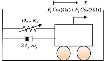
The equation of motion is presented as one degree of freedom damped Duffing oscillator system, which is affected by a bi-frequency harmonic force as shown in Fig. 1. Indicating as the dimensionless displacement of the principle oscillator. The dimensionless equation of motion as presented in [8] is modified as:
where over- dot is the differentiation with respect to time, is the linear damping factor for the main Duffing oscillator, is resonant frequency of the main system, is the coefficient of weak non- linear stiffness, and are the 1:1 and 1:3 resonant harmonic forces amplitudes, respectively, is the external excitation frequency and is the control input.
Fig. 1Schematic graph of the nonlinear oscillator undergone bi-frequency harmonic force
A description of the mathematical technique for PPF, IRC and NIPPF absorbers is supplied as follows. Starting with the technique for the PPF absorber, we have:
where is the state-variable for the PPF controller, , are the damping factor and resonant frequency of the PPF controller, respectively, 0 is the controller gain. We will put in Eq. (1) for 0 in order to close the feedback loop.
Moving to the IRC controller, the model will have the form:
where is the state- variable for the IRC controller, is the lossy integrator’s frequency, 0 is the controller gain. Again, we set in Eq. (1) for 0 to close the feedback loop.
Depending on the two previous controller Eqs. (2) and (3), the NIPPF controller can be described as:
where is the second-order section variable for the NIPPF controller and is the integrating section variable for the NIPPF controller. , are the damping factor and internal frequency for the controller, respectively. 0 and 0 are the gains of controller, is the positive scalar feedback gain of the second- order section, is the positive scalar feedback gain of integrating section, is the lossy integrator’s frequency and is the non-linearity parameter.
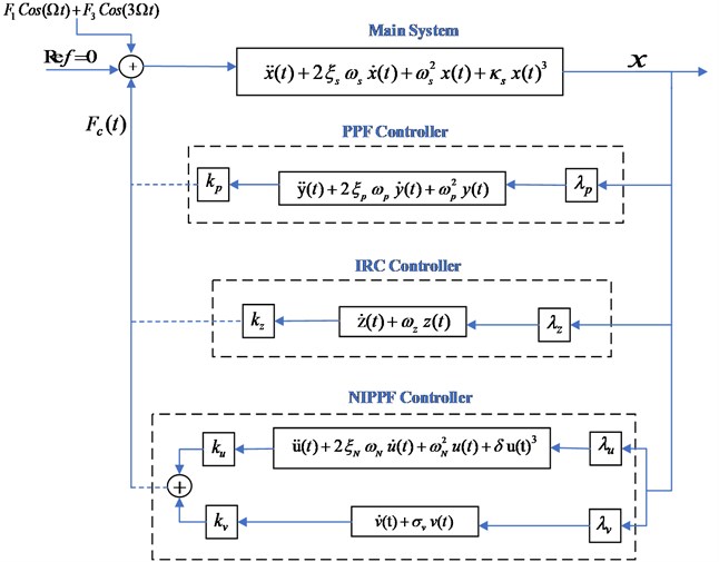
To illustrate the three types for controllers which are connected to a Duffing oscillator system, we presented the following diagram which appeared in Fig. 2.
Fig. 2Schematic graph of the three proposed controllers
2.1. Time history and phase plane by numerical simulation
In this section, Primary resonance ( 0, 0) and super harmonic resonance ( 0, 0) are solved numerically by using the Runge-Kutta fourth-order method (RK-4) with the selected values of the system and the controller parameters introduced in Table 1. This is done for equations that describe a nonlinear dynamic system without and after effecting different types of controls (IRC-PPF-NIPPF) to show the best control.
Table 1Numerical values of the system and NIPPF controller parameters.
Parameter | Value | Parameter | Value | Parameter | Value |
0.003 | –30 | 1 | |||
0.003 | 0.5 | 0.5 | |||
1 | 0.2 | 0.2 | |||
0 | 1 | – | – |
From Fig. 3 to Fig. 6, we have reduced the vibration of the dynamic system of its maximum value to about 96.996 % after using PPF controller at 700 sec and about 1.17 % without any confusion after 200 sec and about 99.183 % after using NIPPF controller at 300 sec. These results are similar in primary resonance (, ) when 0.01, 0and super harmonic resonance case ( , ) when 0, 0.01. This leads to the effectiveness of the absorber ( = steady-state amplitude of the system before controller / steady-state amplitude of the system after controller) is about 33.29 after using PPF controller and about 1.1349 after using IRC controller and about 121.86 after using NIPPF controller for the essential system.
From these results, the NIPPF controller is the best control to suppress the vibration at short time with the good reduction performance and with small chaotic compared to IRC and PPF as shown from Fig. 3 to Fig. 10.
Fig. 3Time estimation of the main system when F1= 0.01, F3= 0 or when F1= 0, F3= 0.01 before controlled system
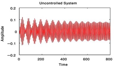
Fig. 4Time estimation of the main system when F1= 0.01, F3= 0 or when F1= 0, F3= 0.01 with PPF controlled only
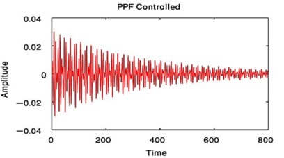
Fig. 5Time estimation of the main system when F1= 0.01, F3= 0 or when F1= 0, F3= 0.01 with IRC controlled only
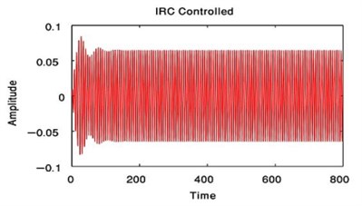
Fig. 6Time estimation of the main system when F1= 0.01, F3= 0 or when F1= 0, F3= 0.01 after NIPPF controlled
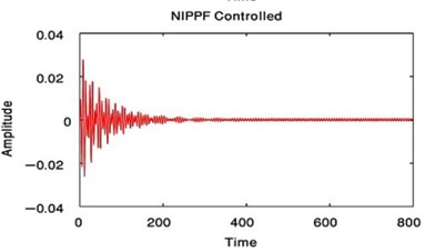
Fig. 7Phase plane of the main system at F1= 0.01, F3= 0 or when F1= 0, F3= 0.01 before controlled system
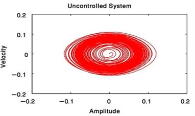
Fig. 8Phase plane of the main system at F1= 0.01, F3= 0 or when F1= 0, F3= 0.01 with PPF controlled only
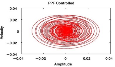
Fig. 9Phase plane of the main system at F1= 0.01, F3= 0 or when F1= 0, F3= 0.01 with IRC controlled only
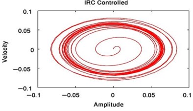
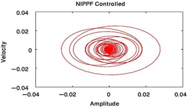
Fig. 10Phase plane of the main system at F1= 0.01, F3= 0 or when F1= 0, F3= 0.01 after NIPPF controlled
3. Mathematical analysis
Applying the multiple scales perturbation technique MSPT, Eqs. (1) and (4) can be solved by imposing the following forms:
where is a small dimensionless parameter of the perturbation and 0 1. ( 0, 1), where the fast-varying time scale will be in the form , and then the slowly varying time scale can be defined as . Therefore, the time derivatives listed such as:
where , 0,1.
One can scale the parameters of Eqs. (1) and (4) as follows , , , , , , , , . This is justified, in order to make all parameters appear in perturbation equations when applying MSPT.
Substituting Eqs. (6)-(10) into Eqs. (1), (4) and comparing the coefficients of identical powers of .
Order ():
Order ():
The differential Eqs. (11) and (12) are assumed to have solutions in the form of:
where the complex functions in are , , indicate the previous complex conjugate terms of Eqs. (17) and (18).
Substituting from Eq. (17) into (13), and solving the resulting ODE, we get the following solution:
where will be determined later. Substitution Eqs. (17)-(19) into Eqs. (14) and (15) leads the general solutions for and can be obtained as:
where the complex functions in are ( 1, 2, ..., 5), and that are presented at appendix. To form the ODE for , substituting Eqs. (19) and (22) into Eq. (16), the solution of this ODE is:
where ( 1, 2, ..., 5) are complex functions in , that are presented at appendix.
The approximate solution of Eqs. (1), (4) can be achieved by exchanging Eqs. (17)-(22) into Eqs. (6)-(8).
Putting the summation of secular terms in the ODE for equivalence to zero, so as to compute the value of . Hence we have:
where is a constant.
3.1. Periodic solution
3.1.1. Primary resonance ( 0, 0)
The steady state solution close to the primary resonance case (, ) is considered from the first order approximation solution. Then, the detuning parameters and will be add such as:
Substituting Eq. (24) into the secular terms elimination, then the following differential equations are obtained:
where ( 1, 2, 3, 4, 5, and 1, 2, 3 are constants (see Appendix).
Using Eq. (9), we will define the derivative of and at the first order with respect to such as:
To find the solution of Eqs. (25), (26), it is appropriate to define , as:
where the steady-state amplitudes are and , and the phases of the polar solutions of the essential system and second - order compensator are , , respectively.
Substituting Eqs. (25), (26), (29), and (30) into Eqs. (27), (28) then equating the real and imaginary terms. Therefore, we abstract the next equations characterizing phases of the response and modulation of the amplitudes:
where , .
Eqs. (31)-(34) are called the autonomous amplitude-phase modulating equations.
3.1.2. Super harmonic resonance ( 0, 0)
The steady state solution close to the super harmonic resonance case (, ) is conducted resulting from the solution of first order approximation. Then, the detuning parameters and will be add such that:
By the same steps of the previous section 3.1.1 with letting and are the steady-state amplitudes, and , are phases that arise in the polar solutions of the essential system and second-order compensator, respectively. Thus, the autonomous amplitude-phase modulating equations are:
where:
and is constants (see Appendix).
3.2. Steady-state oscillations
3.2.1. Primary resonance ( 0, 0)
To get the FRE, the steady state oscillation equations have the following form:
Substituting Eq. (40) into Eqs. (31)-(34), we obtain:
From these equations, we get:
where , , , , ( 1, 2, …, 9) are presented in the Appendix.
Eqs. (48) and (49) are the FRE that are employed to characterize the steady state solutions of system.
3.2.2. Super harmonic resonance ( 0, 0)
Similarly, to obtain the FRE, the steady state oscillation condition have the following form:
Then the FRE in this case are:
where , and , ( 10, 11, …, 16) are presented in the Appendix.
Eqs. (48) and (49) represent the FRE responsible for characterizing the system steady state solutions.
3.3. Stability analysis of the oscillation
3.3.1. Primary resonance ( 0, 0)
To investigate the stability of the nonlinear solution of the achieved fixed points, we must to test the behavior of small deviations (i.e., linearization about the oscillatory point) from the stead state solutions. Thus, we let that:
where , , and are the solutions of Eqs. (34)-(37) and are perturbations which are considered small in comparison to , , and .
Substituting from Eq. (50) into Eqs. (31)-(34), and consideration only the linear terms in , , and , we get the next equations that can be established in the matrix form as:
where the above square matrix is the Jacobian matrix, , 1, 2, 3, 4 and 1, 2, 3, 4 are given in the Appendix. The eigenvalues of the above equations system are specified as:
where means eigenvalues of matrix , , , and are coefficients of Eq. (52). Routh-Hurwitz criterion is employed for testing the stability of the equilibrium solutions. The periodic solution is said to be stable, if the real part of the eigenvalues is negative; else, it is unstable. As indicated by the Routh-Hurwitz criterion, the sufficient and essential conditions for all the roots of Eq. (52) to have negative real parts are:
3.3.2. Super harmonic resonance ( 0, 0)
In addition, to examine the stability of the nonlinear solution of the achieved fixed points, the behavior of small deviations must to be tested (i.e., linearization about the oscillatory point) from the stead state solutions. Thus, we let that:
where , , and are the solutions of Eqs. (36)-(39) and , , , are perturbations which are supposed to be small compared with , , and . we acquire the next equations that can be established in the matrix form as:
where the above square matrix is the Jacobian matrix, , 1, 2, 3, 4 and 1, 2, 3, 4 are given in the Appendix. The eigenvalues of the above equations system are formed as:
As stated by the Routh-Hurwitz criterion, the sufficient and essential conditions for all the roots of Eq. (56) to possess negative real parts are:
4. Results and discussion
4.1. Response curves and effects of different parameters
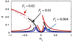
Using MATLAB 7.0 program, the frequency response Eqs. (45), (46) at primary case and Eqs. (48), (49) at super harmonic case have been solved. For the uncontrolled system at 0, the frequency response curve of Duffing oscillator system at primary resonance case are presented as displayed in Fig. 11, where the dashed line is an unstable region and the continuous line is a stable region. At this figure, we observed that, the steady-state amplitude increases during increasing ,increasing the unstable region and bents to left indicating to nonlinear softening spring and jumps phenomenon is occurrence. The difference between the FRC of uncontrolled system at two studied resonance cases has been shown in Fig. 12.
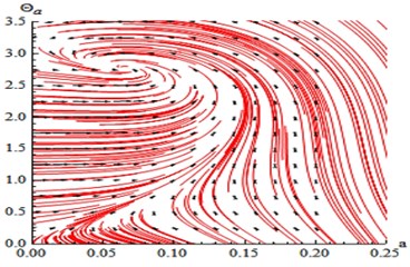
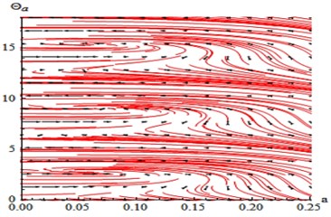
The phase portrait of the uncontrolled system has been shown in Fig. 13 for case (1) at 0, 0, the linear equations , we obtain the critical points obtained from putting 0, 0. Then, the previous linear system can be rewritten in the matrix form where the Jacobian matrix:
We explain the phase portrait classifications for values of the eigenvalues , which obtained from 0. Because of the eigenvalues take the complex formula (, 0, 0), the equilibrium point is classified as the asymptotically stable spiral (spirals in) point at (0.06468, 2.77098+6.28319 k), ( Integers) as in Ref [25].
Fig. 11Effect of different values the external excitation force F1 at F3= 0 of the unabsorbed system when b= 0
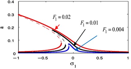
Fig. 12Comparison of the FRC of uncontrolled system at F1= 0.01, F3= 0 and at F1= 0, F3= 0.01
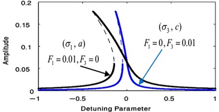
Fig. 13Phase plane of the uncontrolled beam when F1= 0.01, F3= 0, σ1= 0 similarly or at F1= 0, F3= 0.01, σ3= 0
a)
b)
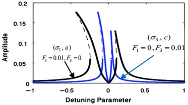
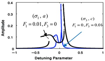
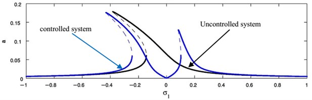
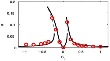
Figs. 14 and 15 show that the FRC for the controlled system at the practical case ( 0, 0), where Fig. 14 displays the steady-state amplitude for the essential system ( against ) and Fig. 15 displays the steady-state amplitude for NIPPF controller ( against ). The comparison of the FRC for the controlled system at two studied cases has been shown in Fig. 15. Also, we observed that the FRC at the primary case resonance is stretched to three times of the FRC at the super harmonic resonances. The comparison between FRC of an uncontrolled system and the system with NIPPF control is presented in Fig. 16. From this figure after using the controller, we obtain a good vibration suppression bandwidth compared to before using the controller.
Fig. 14The FRC of controlled system (a against σ1)
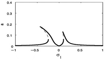
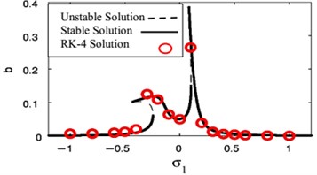
Fig. 15The FRC of controlled system (b against σ1)
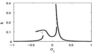
Fig. 16Comparison of the FRC of controlled system at F1= 0.01, F3= 0 and at F1= 0, F3= 0.01
a)
b)
Fig. 17Comparison between the FRC of an uncontrolled system and controlled system
From the above figures, we can discuss the effects of the parameters in one studied resonance case, and the second is similar.
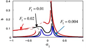
The influences of different parameters on the FRC at the primary case ( against ) and ( against ) are given in Figs. 18 and 19. In Fig. 18(a), (b), we show the FRC of the harmonic force amplitude for the essential system and the restrainer, respectively. Also, this figure shows that the more increasing in the harmonic force amplitude the more bending away of the FRC away from the linear curves. This resulted in jump phenomenon and multi-valued regions. The later can be seen when the solution isn’t equal zero at 0.
The influence of the linear damping on the FRC for the essential system, and the absorber is illustrated in Fig. 18(c), (d), respectively. By increasing the values of the linear damping, the essential system amplitude and the absorber amplitude decreases, the unstable region decrease until all figure becomes stable.
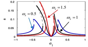
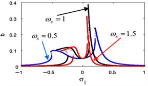
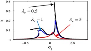
The effects of the linear natural frequency for essential system and controller appears in Fig. 18(e), (f). By decreasing the values of the linear natural frequency, the essential system amplitude decreases, the stable region increases and the vibration suppression bandwidth for the essential system and the controller increases. As a result of that, we knew the small linear natural frequency is suitable for the NIPPF controller to reduction the vibration.
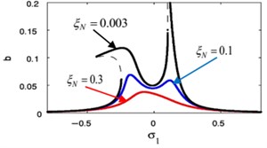
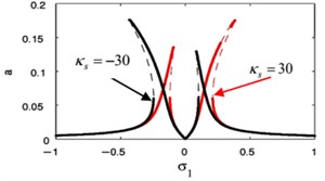
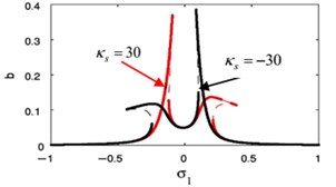
The influence of the weak non-linear stiffness coefficient on the FRC of the essential system and the absorber are shown in Fig. 18(g), (h), respectively. A softening-type spring nonlinearity appeared as a result of the bending to left for the FRC for the essential system and the absorber. In Fig. 18(g) when using the small values of , we find increasing the left peak amplitudes but decreasing the right peak amplitudes for the main system. In contrast to that, when using the small values of , we notice decreasing the left peak amplitudes but increasing the right peak amplitudes for the controller.
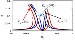
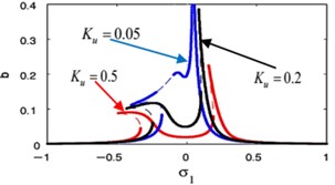
Fig. 18(i), (j) displays the effects of the positive scalar feedback gain on the FRC of the main system and the controller, respectively. Fig. 18(i) displays the increasing of feedback gain , the vibration suppression bandwidth become wider and the right peak amplitudes are monotonic increasing for the main system amplitude. In Fig. 18(j) when the solution isn’t equal zero at 0 with the increasing of feedback gain , the controller amplitude will decrease.
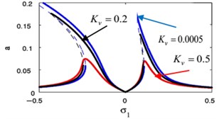
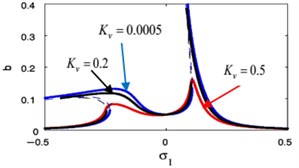
The effects of the integrating gain on the FRC of the main system and the controller are showed in Fig. 18(k), (l), respectively. This figure appears the decreasing of peak amplitudes for the main system and the absorber, the increasing in stable region when increasing of integrating gain.
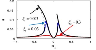
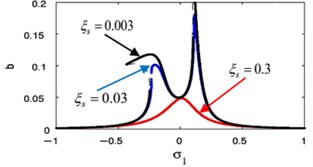
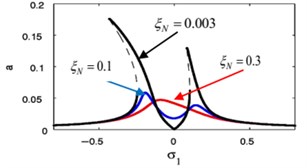
Fig. 18(m), (n) indicates that for growing values of the linear damping for the absorber , the steady-state amplitudes for the essential system and the controller are reduced, and the unstable region is decreased until total figure become stable. Also, we noticed that at 0 the amplitude of the main system moving away from zero, which is supposed to reach zero at primary resonance case that occurs at 0, therefore, it is preferable to take a small value for the variable .
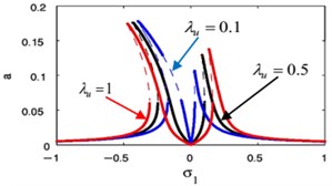
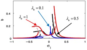
Fig. 18(o) illustrates that for large values of the controller gain for the PPF control , the vibration suppression bandwidth is wider and the right peak amplitudes are monotonic increasing for the main system amplitude. Fig. 18(p) displays that the absorber peak amplitudes increases.
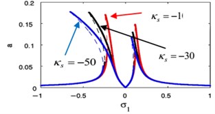
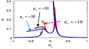
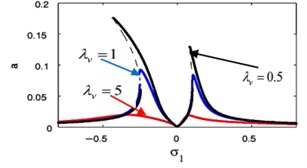
The effects of the controller gain of the IRC control on the FRC of the essential system and the absorber are shown in Fig. 18(q), (r), respectively. By increasing the Controller gain for the IRC control, the peak amplitudes of the essential system and the absorber decrease, the unstable region decrease until all figure become stable.
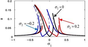
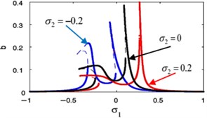
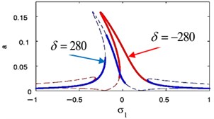
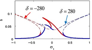
Fig. 18(s), (t) shows the FRC of the essential system and the absorber by varying the value of the detuning parameter . Now, we notice that for –0.2, the steady-state amplitudes of essential system and the absorber are minimize when –0.2. For 0, the steady-state amplitudes of essential system and the absorber are minimize when 0. Finally, for 0.2, the steady-state amplitudes of essential system and the absorber are minimize when 0.2. Accordingly, the steady-state amplitudes of essential system and absorber are minimize when i.e. ().
Fig. 19(a), (b) shows that when changing the sign of weak non-linear stiffness coefficient , the amplitude for the essential system and the amplitude of absorber is curved to the right denoting a hardening-type spring nonlinearity.
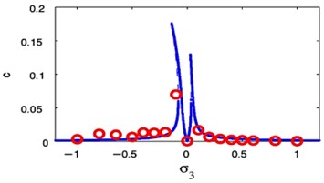
The influence of the nonlinear term coefficient at 0.009, 0 on FRC of the essential system and the absorber is presented in Fig. 20. Moreover, varying versus the amplitude for the essential system and amplitude of the absorber , are depicted in Figs. 21 and 22 respectively. Therefore, the steady-state amplitudes of base system and absorber is minimized when 0.
Fig. 18Effective of various parameters on the FRC
a)
b)
c)
d)
e)
f)
g)
h)
i)
j)
k)
l)
m)
n)
o)
p)
q)
r)
s)
t)
Fig. 19The frequency response curve when changing the sign of κs
a)
b)
Fig. 20Sensitivity of the frequency response curve when with change its sign at F1= 0.009, F3= 0
a)
b)
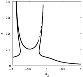
Fig. 21Effective of σ2 on the FRC (a against σ2)
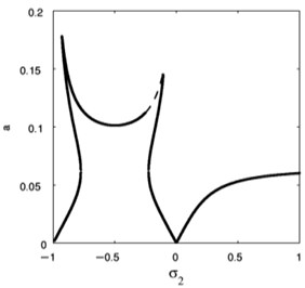
Fig. 22Effective of σ2 on the FRC (b against σ2)
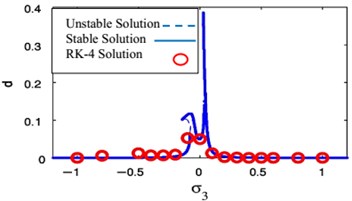
We observed the rapprochement between the analytical and the numerical solution of the FRC as in Figs. 23 and 24 in two resonance cases of study, respectively. From these figures, all predictions based on evidence of the analytical solution are at extremely valid coincidence with the numerical solution.
Fig. 23FRC and numerical solutions at F1= 0.01, F3= 0
a)
b)
Fig. 24FRC and numerical solutions F1= 0, F3= 0.01
a)
b)
4.2. Comparison between time response solutions of the MSPT and the RK-4 methods
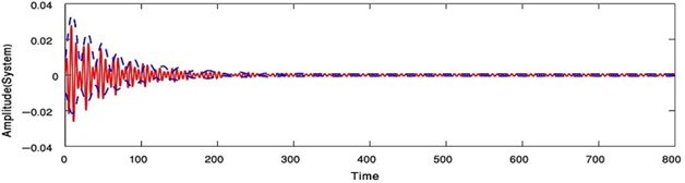
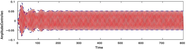
Applying the condition for a steady-state solution, that is, 0 at the primary resonance case or 0 at the super harmonic resonance case, the comparison between the numerical solutions of Eqs. (1) and (4) for NIPPF control and the analytical solutions given by Eqs. (31)-(34) in case of the primary resonance case or Eqs. (36)-(39) in case of the super harmonic resonance has been declared as in Fig. 25. The dashed lines indicate the modulation of the amplitudes for the generalized coordinate , . On the other hand, the continuous lines represent the time history of vibrations, which acquired numerically as solutions of the original equations of the system with NIPPF controller. From this figure, we found that the two studying cases of resonance are applicable to each other at the steady state solution. Also, there is a good agreement between analytical and numerical solutions.
Fig. 25Time response where () analytic solution () numerical solution at F1= 0.01, F3= 0 with the primary resonance case Ω=ωs, ωN= ωs or at F1= 0, F3= 0.01 with the super harmonic resonance case (Ω=ωs/ 3, ωN=ωs)
a)
b)
5. Comparison between the previous works and this work
In a previous work [8], the authors studied the influence of the use of the NES for passive control vibration under bi- frequency harmonic force through considering and the (non-dimensional) displacement of the principle non- linear oscillator. They applied MSHBT, to find the relevant amplitude modulation equations. Three situations have been investigated for the external harmonic excitation: 1:1 resonance, 1:3 resonances, and concurrent 1:1 and 1:3 resonances. Analytical and numerical solutions, for the principle non- linear oscillator are displayed at primary, sub harmonic and primary and sub harmonic resonance.
Firstly, we adjusted the equation of Ref. [8] by considering only (non-dimensional) displacement of the principle non- linear oscillator. We utilized NIPPF absorber was offered as the best controller compared to the other controllers to control the vibration system as shown in this paper.
Secondly, we applied the MSPT to get a solution of the studied system and examined the stability of this system.
Finally, we have succeeded in reducing the steady-state amplitude of the main system to 99.183 % after using NIPPF absorber from its value before absorber. For obtaining the effective NIPPF controller, we have found that it is necessary tuning the controller natural frequency to the external excitation frequencies ().
The authors declared no potential conflicts of interest with respect to the research, authorship, and/or publication of this article.
6. Conclusions
In this article, the numerical comparison of the evolution of time between three different types of control, which are IRC, PPF and NIPPF controllers on the basic system. We found that the best in terms of reducing vibration at a high rate and after a short time is NIPPF controller. Then, a Duffing oscillator system connected to NIPPF was introduced with three coupled differential equations. These equations have been solved analytically by using MSPT approximation. The FRE has been obtained near the primary resonance and super harmonic resonance. After that we have investigated the effects of the parameters to present the amplitude performance of the system and NIPPF. The stability study is completed to define the stable boundary of the control variables.
From this research, the highlighted points can be summarized as following:
1) By using NIPPF controller, the steady-state amplitude is decreased to 99.18 % from its value before control, which proved that this control is the best compared to use of the IRC or PPF controllers.
2) The effectiveness of the absorber is about 33.29 when using PPF controller and about 121.86093 after using NIPPF controller for the main system.
3) The amplitudes of a Duffing system and the controller are increased when increasing the values of and .
4) At decreasing the value of, and , the amplitude of the main structure and the controller are increased.
5) For increasing the values of , and , the amplitude of the main structure decreased and the amplitude of the controller increased.
6) The FRC of Duffing system and the controller are curved to the right denoting a hardening-type spring nonlinearity when changing the sign value of .
7) The best performance for the amplitude vibration reduction which reach to zero when () and similarly when ().
8) There are good agreements when make a comparison between the approximate and the numerical solutions at time history and the FRC as presented in Figs. 23, 24 and 25 at two cases of study, respectively.
References
-
Frýba L. Vibration of Solids and Structures under Moving Loads. Springer Science and Business Media, 2013.
-
Yang Y., Ding H., Chen L.-Q. Dynamic response to a moving load of a Timoshenko beam resting on a nonlinear viscoelastic foundation. Acta Mechanica Sinica, Vol. 29, Issue 5, 2013, p. 718-727.
-
Jung W., Noh I., Kang D. The vibration controller design using positive position feedback control. International Conference on Control, Automation and Systems, Gwangju, Korea, 2013.
-
El Ganaini W.-A., Saeed N. A., Eissa M. Positive position feedback (PPF) controller for suppression of nonlinear system vibration. Nonlinear Dynamics, Vol. 72, 2013, p. 517-537.
-
Ghadiri M., Rajabpour A., Akbarshahi A. Nonlinear forced vibration analysis of nanobeams subjected to moving concentrated load resting on foundation considering thermal and surface effects. Applied Mathematical Modelling, Vol. 50, 2017, p. 676-676.
-
Russell D., Fleming A. J., Aphale S. S. Improving the positioning bandwidth of the integral resonant control scheme through strategic zero placement. The International Federation of Automatic Control, Vol. 19, 2014, p. 24-29.
-
Omidi E., Mahmoodi S. N. Sensitivity analysis of the nonlinear integral positive position feedback and integral resonant controllers on vibration suppression of nonlinear oscillatory systems. Communications in Nonlinear Science and Numerical Simulation, Vol. 22, 2015, p. 194-166.
-
Zulli D., Luongo A. Control of primary and sub harmonic resonances of a Duffing oscillator via non-linear sink. International Journal of Non-linear Mechanics, Vol. 80, 2016, p. 170-182.
-
Eissa M., Saeed N. A. Nonlinear vibration control of a horizontally supported Jeffcott-rotor system. Journal of Vibration and Control, 2017, https://doi.org/10.1177/1077546317693928.
-
Saeed N. A., Kamal M. Active magnetic bearing-based tuned controller to suppress lateral vibrations of a nonlinear Jeffcott rotor system. Nonlinear Dynamics, Vol. 90, 2017, p. 457-478.
-
Eissa Kandil M. A., El Ganaini W.-A., Kamel M. Vibration suppression of a nonlinear magnetic levitation system via time delayed nonlinear saturation controller. International Journal of Non-Linear Mechanics, Vol. 72, 2015, p. 23-41.
-
Hilla T. L., Neilda S. A., Waggb D. J. Comparing the direct normal form method with harmonic balance and the method of multiple scales. Procedia Engineering, Vol. 199, 2017, p. 869-874.
-
Amer Y. A., El Sayed A.-T., Kotb A. A. Nonlinear vibration and of the Duffing oscillator to parametric excitation with time delay feedback. Nonlinear Dynamics, Vol. 85, Issue 4, 2016, p. 2497-2505.
-
Bauomy H. S., El Sayed A.-T. Active control of a rectangular thin plate via negative acceleration feedback. Journal of Computational and Nonlinear Dynamics, Vol. 11, Issue 4, 2016, p. 041025.
-
Zhao H., Sun M., Deng W., Yang X. A new feature extraction method based on EEMD and multi-scale fuzzy entropy for motor bearing. Entropy, Vol. 19, Issue 1, 2017, p. 14.
-
Deng W., Yao R., Zhao H., Yang X., Li G. A novel intelligent diagnosis method using optimal LS-SVM with improved PSO algorithm. Soft Computing, 2017, https://doi.org/10.1007/s00500-017-2940-9.
-
Deng W., Zhao H., Zou L., Li G., Yang X., Wu D. A novel collaborative optimization algorithm in solving complex optimization problems methodologies and application. Soft Computing, Vol. 21, 2017, p. 4387-4398.
-
Deng W., Zhao H., Yang X., Xiong J., Sun M., Li B. Study on an improved adaptive PSO algorithm for solving multiobjective gate assignment. Applied Soft Computing, Vol. 59, 2017, p. 288-302.
-
Deng W., Zhang S., Zhao H., Yang X. A novel fault diagnosis method based on integrating empirical wavelet transform and fuzzy entropy for motor bearing. IEEE Access, Vol. 6, Issue 1, 2018, p. 35042-35056.
-
Deng W., Zhao H., Liu J., Yan X., Li Y., Ding C. An improved CACO algorithm based on adaptive method and multi-variant strategies. Soft Computing, Vol. 19, Issue 3, 2015, p. 701-713.
-
Deng W., Chen R., He B., Liu Y., Ding C., Yin L., Guo J. A novel two-stage hybrid swarm intelligence optimization algorithm and application. Soft Computing, Vol. 16, Issue 10, 2012, p. 1707-1722.
-
Deng W., Chen R., Goa J., Song Y., Xu J. A novel parallel hybrid intelligence optimization algorithm for a function approximation problem. Computer and Mathematics with applications, Vol. 63, Issue 1, 2012, p. 325-336.
-
Deng W., Yang X., Zou L., Wang M., Liu Y., Li Y. An improved self-adaptive differential evolution algorithm and its application. Chemometrics and intelligent laboratory systems, Vol. 128, 2013, p. 66-76.
-
Zhao H. M., Li D. Y., Deng W., Yang X. H. Research on vibration suppression method of alternating current motor based on fractional order control strategy. Journal of Process Mechanical Engineering, Vol. 231, Issue 4, 2017, p. 786-799.
-
Abourabia A. M., Hassan K. M., Selima E. S. Painleve analysis and new analytical solutions for compound KdV-Burgers equation with variable coefficients. Canadian Journal of Physics, Vol. 88, Issue 4, 2010, p. 211-221.
Cited by
About this article

