Abstract
The formation of super-directivity of an acoustic array is firstly analyzed to construct a general mathematical model of the array with super-directivity and maximum signal-to-noise ratio (SNR). Then the numerical simulation on the super-directivity of the array is carried out for the arrays with different shapes, element number and apertures. It shows that, circular array with regular shape and Archimedean spiral array with irregular shape have optimum directivity.
1. Introduction
Super-directivity of acoustic array has been widely applied in measurement, identification and analysis of noise sources. However, existing researches in the super-directivity proceed from modeling signal-to-noise ratio (SNR) [1] and or incident field [2], without forming a complete mathematical model. Most of the investigations focus on regular arrays, such as linear and spherical ones [3-5]. Regular arrays (e.g., circular, square) and irregular arrays (e.g., Archimedes spiral) are often encountered in microphones [6], but rarely involved in the studies. In this paper, the formation process of the super-directivity of acoustic array is analyzed firstly, afterward, the mathematical model of the array with super-directivity and maximum SNR is also established. Then, the super-directivities of different arrays are analyzed numerically by using directivity index, maximum SNR, beam width of sound wave.
2. Formation and mathematical modeling of super-directivity
2.1. The forming process
A microphone array is constructed by a number of microphone-array elements that are arranged in order or disorder. Both received, and the emitted signals of the elements affect obviously on the transmittal property, especially on the directivity of the array. The forming process of the super-directivity of an acoustic array with maximum SNR is shown in Fig. 1.
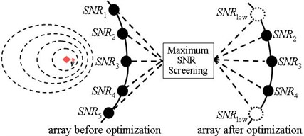
Fig. 1(a) illustrates the process of an acoustic array for identifying the still sound source and screening out the elements. Because the source is still, and its sound energy radiates into surrounding uniformly, the output from each of the elements has basically identical SNR, and thus the number of array elements before and after the screening keeps the same. Fig. 1(b) illustrates the process of an acoustic array for identifying the directivity of the moving sound source. Since the source is in motion, its sound energy is focused into the moving direction, each of the elements receives different amount of sound energy, which results in the output from each element with different SNR, and thus the elements of the array are screened out.
The rule for the screening is that: suppose the SNR of each element is , as shown in Fig. 1, which are labeled as , ,…, . From the SRN formula, can be expressed as:
where is the effective power of the signal received by the element, and is the effective power of the output noise of the element. Assume that, of each element is equal and the maximum SNR of the single element in a super-directional acoustic array is set to be in dB. If , the directivity of corresponding element to the sound source is relatively strong, the element should be then retained; If , indicating that the location of corresponding element has poor directivity to the source, and thus should be removed. All the retained elements after such screening process can be used to form an acoustic array with super-directivity [7].
Fig. 1Process of optimizing the array with maximum SNR
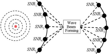
a) Still sound source
b) Moving sound source
2.2. Mathematical model
In process of forming the super-directivity of an acoustic array, the elements and SNR of the array have critical influence on the directivity. In view of this, the mathematical modeling of forming super-directivity with maximum SNR is given here. For an acoustic array with elements in uniform spatial sound field, its normalized signal vector, which is called steering vector in wave-beam forming and used to solve for positioning sound source, is supposed to be:
where , (0,..., ) is the sound-path-difference of the signal of the -th microphone element as a referential point, and is sound wave number. Therefore, the normalized covariance-matrix of the source in uniform spatial field should be:
where is the noise pick-up vector of microphone array, is the noise variance, is the mathematical expectation, star * and letter denote conjugation and transpose operations of the vectors, respectively, and:
Eq. (4) is the spatial correlation coefficient in-between the -th and -th elements in an isotropic and uniform spatial sound field, and is the wavelength of incident sound wave. Therefore, SNR of the output from the array, denoted by , can be determined by:
where and are the acoustic and noise components in output signal respectively, represents the element weighting vector, denotes the sound source strength, , which represents input SNR at the element. Then, the directivity factor of the array is:
Because is a positive definite matrix, it can be decomposed into the product of two equal Hermitian matrices, i.e., where denotes the directional matrix of the array. Introduce a vector , then:
where . Then, finding the maximum value of becomes the issue to find the maximum eigenvalue of , that is, . Then , and the optimum weighting factor . Rewrite the form of as , . The rank of can be solved to be 1. It has only one non-zero eigenvalue , which is also the maximum eigenvalue. Thus:
Since , obviously, will be one of the eigen-vectors of . Meanwhile, in the equation should be , that is, the maximum directivity factor is Correspondingly, , i.e.:
Thus, a general mathematical model for the super-directivity of an acoustic array with maximum SNR has been obtained here to this point. The general model provides the basis for measuring the field directivity of a moving sound source, and further determines the evaluation parameters, such as directivity index, maximum SNR and wave-beam width, which are used to analyze and study the super-directivity of an acoustic array, as seen next.
3. Analysis on directive characteristics
3.1. Effect of element shape on the directivity
3.1.1. Numerical analysis on directivity of the array with regular shape
Using the parameters of evaluating super-directivity, the directivities of following two regular planar arrays with different shapes are compared here. Under the conditions of the same parameters, such as aperture, number of elements, and spacing in-between elements, etc., the directivities of rectangular and circular microphone arrays are analyzed comparatively.
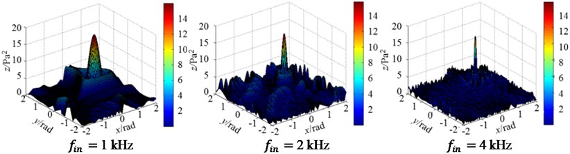
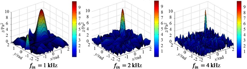
Conditions: Incident angle of gradient and incident directional angle from the sound source are 45° and 45° respectively; Incident sound wave frequencies are set to be 1 kHz, 2 kHz and 4 kHz; Element number of the microphone array is set to be 32; Diagonal length of the rectangular array is set to be 2 m, and radius of the circular array is 1 m.
Via simulation, the acoustic energy output from the array, described by square sound pressure in Pa2, are provided. Specifically, the amplitude distributions of three-dimensional response functions of the two arrays at incident frequencies 1 kHz, 2 kHz and 4 kHz, respectively, are shown in Fig. 2. Where, -, -, and -axes represent the incident angle of gradient, incident directional angle, and amplitude of output acoustic energy, respectively, for the array. From these results, it can be concluded that the circular microphone array has better directivity.
Fig. 2Three-dimensional magnitude distribution patterns of regular arrays at 3 incident frequencies
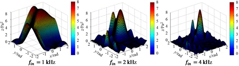
a) Rectangular array (2 m)
b) Circular array (1 m)
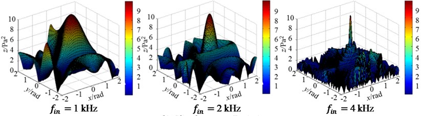
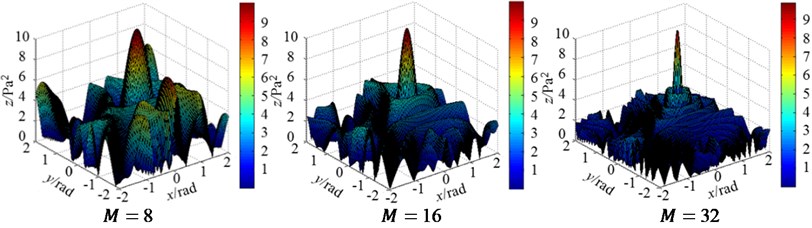
Fig. 3Three-dimensional magnitude distribution patterns of irregular arrays at 3 incident frequencies
a) Archimedes spiral array (2 m)
b) Logarithmic spiral array (1 m)
3.1.2. Numerical analysis on directivity of the array with irregular shape
In case of irregular arrays, here takes Archimedes and logarithmic spiral arrays as examples. All other conditions are right the same as that of Section 3.1.1, including the incident sound wave frequencies, and the aperture of the array is still fixed to be 2 m. The directivity patterns of Archimedes and logarithmic spiral arrays are shown in Fig. 3. It can be concluded from Fig. 3 that Archimedes spiral array as a irregular one has stronger directivity.
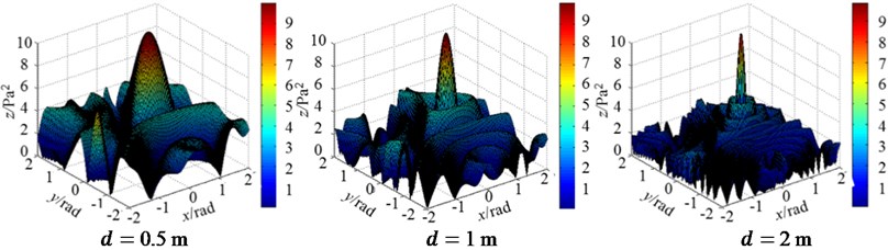
Fig. 4Three-dimensional magnitude distribution patterns of two arrays changing with element number
a) Regular circular array ( 1 m)
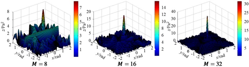
b) Irregular Archimedes spiral array (1 m)
Fig. 5Three-dimensional magnitude distribution patterns of two arrays changing with element aperture
a) Regular circular array (32)
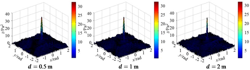
b) Irregular Archimedes spiral array (32)
3.2. Effect of element number and aperture on directivity
To study the effect of element number and aperture on the directivity of an acoustic array, here fix the aperture but change the number to simulate the directivity at first. Under the same conditions, the directivity patterns of the regular circular and irregular Archimedes spiral arrays, with the same element aperture 1 m, but three different element number 8, 16 and 32, respectively, are shown in Fig. 4. Then, fix the element number of the two arrays, 32, but change their aperture to be 0.5, 1 and 2 m respectively. The simulated directivity patterns of the regular circular and irregular Archimedes spiral arrays are shown in Fig. 5.
It can be concluded From Figs. 4-5 that, under the same conditions:
a) The more the number of elements is, the better the directivity of an acoustic array will be. In case of identical number, Archimedes spiral array shows better directive performance;
b) The larger the aperture of a microphone array is, the smaller the width of the main-lobe in the pattern will be. Simultaneously, the magnitude of the side-lobe changes its amplitude greater and tends to decrease the amplitude. The directivity of the array is thus to be enhanced as the aperture becomes larger.
4. Conclusions
The main conclusions of this study are as follows:
1) The super-directivity of an acoustic array is influenced by the frequency of incident sound wave, element number and aperture of the array.
2) Circular microphone array shows better directivity in the arrays with regular shapes and has simple configuration. Its data is easily processed and computed. While, Archimedean spiral array in arrays with irregular shapes shows even better directivity than that of the circular one.
3) The acoustic array with super-directivity has such properties as maximum SNR, narrow main-lobe width of wave-beam, and good side-lobe suppression.
References
-
Lee P. L., Wang J. H. The simulation of acoustic radiation from a moving line source with variable speed. Applied Acoustics, Vol. 71, 2010, p. 931-939.
-
Wang J. H., Lee P. L. Determination of the acoustic position vector of a moving sound source with constant acceleration motion. Engineering Analysis with Boundary Elements, Vol. 33, 2009, p. 1141-1144.
-
Widrow B., Mantey P. E., Griffiths L. J. Adaptive antenna system. Proceedings of the IEEE, Vol. 55, 1967, p. 2143-2158.
-
Capon J. High resolution frequency-wavenumber spectrum analysis. Proceedings of the IEEE, Vol. 57, 2007, p. 1408-1418.
-
Cho Y. T., Roan M. J. Adaptive near-field beam forming techniques for sound source imaging. The Journal of the Acoustical Society of America, Vol. 3, 2009, p. 944-957.
-
Strobel N., Spors S., Rabenstein R. Joint audio-video object localization and tracking. IEEE Signal Processing Magazine, Vol. 18, Issue 1, 2001, p. 22-31.
-
Potamitis I., Chen H. M., Tremoulis G. Tracking of multiple moving speakers with multiple micro-phone arrays. IEEE Transactions on Speech and Audio Processing, Vol. 12, Issue 5, 2004, p. 520-529.
About this article

This work was supported by the National Natural Science Foundation of China (Grants No. 61671262 and No. 51475211).
