Application of the energy finite element analysis to vibration of beams with stepped thickness and variable cross-section

Lin, Zhili; Chen, Xiliang; Zhang, Bo

doi:10.21595/jve.2018.19625

Journal of Vibroengineering

Browse Journal

Submit article

Published: 30 September 2018

Check for updates

Application of the energy finite element analysis to vibration of beams with stepped thickness and variable cross-section

Zhili Lin¹

Xiliang Chen²

Bo Zhang³

^{1, 2}University of Chinese Academy of Sciences, Beijing, 100049, China

^{1, 2, 3}Ningbo Institute of Material Technology and Engineering, Chinese Academy of Sciences, Ningbo, 315201, China

³School of Mechatronic Engineering and Automation, Shanghai University, Shanghai, 200072, China

Corresponding Author:

Xiliang Chen

Cite the article Download PDF

Downloads 1632

WoS Core Citations 4

CrossRef Citations 3

Abstract

Energy finite element analysis (EFEA) has been developed to compute the energy distribution of vibrating structures. The method adopts the energy density as the basic variable of differential equation. The energy density can be used to analyze the behavior of vibrating beams. Firstly, an EFEA equation is obtained from the classical displacement equation. In the applications of uniform and non-uniform beams, the EFEA results are compared with the analytical and FEA results. Secondly, a junction formulation solving the discontinuity problem of energy density at the junction of two beams with stepped thickness is proposed. The EFEA equation combined with junction formulation is used to solve the energy transmission problem of the coupling beams with stepped thickness and variable cross-section. The smoothed results of coupling beams are achieved, and the differences of energy density at the junctions are analyzed. The feasibility of the EFEA approach is validated by using several design examples under the various frequencies and structural damping loss factors.

1. Introduction

In mid-to-high frequency range, the prediction of complex structural response using traditional finite element analysis (FEA) approach is time-consuming and costs a plenty of resources because the wavelength decreases when the analysis frequency increases [1, 2]. For this reason, statistical energy analysis (SEA) approach was proposed and widely applied to the industrial applications [3, 4]. SEA can seize the global energy variable of every divided system, but this approach cannot yield the space information of energy variable for every system [5, 6].

Energy finite element analysis (EFEA) approach was recently proposed for the prediction of structural response in mid-to-high frequency range [7, 8]. Comparing with SEA approach, EFEA method can yield the space information of energy variable for every system and can use the numerical solution technique like FEA approaches. In the EFEA approach, the differential equation in terms of energy variation is formulated. The equation is developed for all wave bearing domains of every system. The results of energy density vary exponentially with the spatial position. Thus, a small number of finite elements can seize the energy variables. Comparing with FEA approach, the EFEA approach only uses less computational resources and a short time that affects the design cycles of mechanical products [9].

There is a little difference between the energy relationships proposed by Nefske [1] and by Wohlever [4]. Nefske relationship is associated with local variables, but Wohlever relationship is associated with space-averaged variables [10]. Wohlever relationship is utilized to obtain the energy finite element equation in current investigation. When the wavelength is far less than the structural dimension, the far field assumption is valid enough for the response prediction of vibrational structures in mid-to-high frequency range [11-13].

In this paper, the EFEA approach is extended to the coupled beams with stepped thickness and variable cross-section in mid-to-high frequency range. It is less investigated on the published documents. Firstly, an EFEA equation is derived from the classical displacement equation for predicting the distribution of energy density for uniform and non-uniform beams. The deriving equation employs the energy variable to seize the vibration behavior of uniform and non-uniform beams. The obtained results of energy density are compared with the analytical and FEA results. Secondly, a junction equation in terms of group speeds and energy transfer coefficients is obtained. This junction equation is used to solve the problem of discontinuous nodal values of energy density in the junctions and applied to coupled beams with stepped thickness. Then, the smoothed results of coupled beams are available, and the differences between the left and right nodal values of energy density at the junctions are analyzed. A convergence study of the EFEA approach is achieved and confirmed. The feasibility of the developed EFEA approach is validated by using several design examples under the various excitation frequencies and hysteresis damping loss factors.

2. Basic theory

2.1. Analytical equation

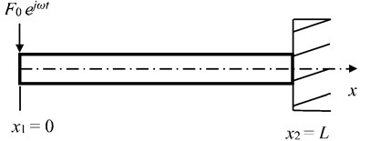
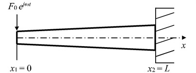
The motion equation for flexural waves in a uniform Euler-Bernoulli beam shown in Fig. 1, excited by a general forcing function is:

1

E I \frac{\partial^{4} w (x, t)}{\partial x^{4}} + ρ S \frac{\partial^{2} w (x, t)}{\partial x^{2}} = F (x, t),

where $w (x, t)$ denotes a complex displacement in the transverse direction in the time $t$ , $E I$ denotes a bending stiffness, $ρ S$ denotes a density for a unit length, $F (x, t)$ denotes a distributed forcing function in the direction $x$ in the time $t$ for a unit length.

For this investigation, an excitation will be modeled as a harmonic point force. This excitation is a transverse force imposing perpendicular to the neutral axis and is defined mathematically as:

2

F (x, t) = F_{0} δ (x - x_{0}) e^{j ω t},

where $F_{0}$ is the magnitude of forcing function, $ω$ is the excitation frequency, $j$ is the imaginary number, $δ (x - x_{0})$ is a dirac delta function defined as:

\{\begin{array}{l} δ (x - x_{0}) = 0, x \neq x_{0}, \\ \int_{- \infty}^{\infty} δ (x - x_{0}) d x = 1 . \end{array}

From Eq. (1), a general solution can be obtained as:

3

w (x, t) = [A e^{- j k x} + B e^{- k x} + C e^{j k x} + D e^{k x}] e^{j ω t},

where the constants $A$ , $B$ , $C$ and $D$ are complex displacement amplitudes which can be determined from boundary conditions, $k$ denotes a flexural wavenumber, $ω$ is the excitation frequency. For transversely vibrating beams, the boundary conditions of displacement, slope, moment, and shear force are allowed. In Eq. (3), the first term $A e^{- j k x}$ denotes a forward propagating flexural wave, the second term $B e^{- k x}$ denotes a forward decaying nearfield, the third term $C e^{j k x}$ denotes a backward propagating flexural wave, and the fourth term $D e^{k x}$ denotes a backward decaying nearfield. The flexural wavenumber $k$ is defined as:

4

k = {[\frac{ω^{2} ρ S}{E I}]}^{1 / 4} .

For a beam excited by harmonic point force, the time-averaged energy density of flexural waves is:

5

⟨e⟩ = \frac{1}{4} E I (\frac{\partial^{2} w}{\partial x^{2}} \frac{\partial^{2} w^{*}}{\partial x^{2}}) + \frac{1}{4} ρ S (\frac{\partial w}{\partial t} \frac{\partial w^{*}}{\partial t}),

where the first term is the time-averaged potential energy density item, the second is the time-averaged kinetic energy density item, $w^{*}$ is the complex displacement, $\partial^{2} w / \partial x^{2}$ is the conjugate of the angular displacement, $\partial^{2} w^{*} / \partial x^{2}$ is the complex conjugate of the angular displacement, $\partial w / \partial t$ is the conjugate of the transverse velocity, $\partial w^{*} / \partial t$ is the complex conjugate of the transverse velocity. Eq. (5) is referred to as the “exact” results of energy density for Euler-Bernoulli beams.

Fig. 1A free-clamped uniform beam

2.2. Energy finite element equation

In the far field, the energy equation of the vibrating Euler-Bernoulli beam with a flexural excitation can be expressed as [4]:

6

- \frac{c_{g}^{2}}{ω η} \frac{d^{2} ⟨\bar{e}⟩}{d x^{2}} + ω η ⟨\bar{e}⟩ = ⟨π_{i n}⟩,

where $c_{g}$ denotes a group speed of flexural wave [12], $η$ denotes a structural damping, $ω$ denotes an analysis frequency, $⟨\bar{e}⟩$ denotes an item of energy density in terms of time- and space-averaged, $⟨π_{i n}⟩$ denotes an input power item [14] defined as:

7

⟨π_{i n}⟩ = \{\begin{array}{l} π_{i n}^{1} & \dots & π_{i n}^{m} \end{array}\},

8

π_{i n}^{i} = \frac{1}{2} | F_{0} |^{2} R e a l \{\frac{1}{Z_{\infty}}\},

9

Z_{\infty} = \frac{1}{2} ρ S c_{b} (1 + j),

where $i$ denotes a number among 1, ..., $m$ , $F_{0}$ denotes a magnitude of harmonic point force, “Real” in Eq. (8) denotes exacting the real part of a quantity, $Z_{\infty}$ denotes an input impedance [15], $ρ$ denotes the density of beam material, $S$ denotes an area of cross-section, $c_{b}$ denotes the phase speed of the flexural wave, $j$ denotes an imaginary number.

An EFEA equation to predict the structural response of vibrational beams will be achieved from Eq. (6). References [1, 3] report that the EFEA equation can be solved numerically, and the solution process is like FEA methods. From the Eq. (6), a weak form is obtained as:

10

\int ϕ^{T} \{- \frac{c_{g}^{2}}{ω η} \nabla^{2} ⟨\bar{e}⟩ + ω η ⟨\bar{e}⟩ - ⟨π_{i n}⟩\} d x = 0,

where $ϕ^{T}$ denotes a test function transpose. Applying the integral subsection integration approach, an expression can be available as:

11

\int ϕ^{T} \{- \frac{c_{g}^{2}}{ω η} \nabla^{2} ⟨\bar{e}⟩\} d x = \int \{- \frac{c_{g}^{2}}{ω η} \frac{d ϕ^{T}}{d x} \frac{d ⟨\bar{e}⟩}{d x}\} d x + ϕ^{T} {[\frac{c_{g}^{2}}{ω η} \frac{d ⟨\bar{e}⟩}{d x}]}_{x_{i}}^{x_{i + 1}},

where $x_{i}$ denotes left value of a beam element, and $x_{i + 1}$ denotes right value of a beam element.

Eq. (11) is substituted into Eq. (10), an expression is:

12

\int \{\frac{c_{g}^{2}}{ω η} \frac{d ϕ^{T}}{d x} \frac{d ⟨\bar{e}⟩}{d x}\} d x + \int \{ω η ⟨\bar{e}⟩\} d x = \int \{ϕ^{T} ⟨π_{i n}⟩\} d x + ϕ^{T} {[\frac{c_{g}^{2}}{ω η} \frac{d ⟨\bar{e}⟩}{d x}]}_{x_{i}}^{x_{i + 1}},

where first item denotes a stiffness matrix, second item denotes a mass matrix, third item denotes an input power, and the fourth item denotes an energy flow across boundaries. The derivation of EFEA equation is finished by employing Galerkin weighted residual approach. In the Eq. (12), the energy density and the test function can be expressed as:

13

⟨\bar{e}⟩ = \sum_{i = 1}^{m} N_{i} e_{i},

14

ϕ = [\begin{array}{l} N_{1} (x) & \cdot \cdot \cdot & N_{m} (x) \end{array}],

where $N_{i}$ is a shape function of a beam element, $i$ denotes a number among 1, ..., $m$ .

Finally, the EFEA equation of a beam element is formed as:

15

K^{(e)} e^{(e)} = π_{i n}^{(e)} + B^{(e)},

where:

16

K^{(e)} = \int \{\frac{c_{g}^{2}}{ω η} \frac{d ϕ^{T}}{d x} \frac{d ϕ}{d x}\} d x + \int \{ω η ϕ\} d x,

17

e^{(e)} = \{\begin{array}{l} e_{1} \\ ⋮ \\ e_{m} \end{array}\},

18

π_{i n}^{(e)} = \int \{ϕ^{T} ⟨π_{i n}⟩\} d x,

19

B^{(e)} = ϕ^{T} {[\frac{c_{g}^{2}}{η ω} \frac{d ϕ}{d x}]}_{x_{i}}^{x_{i + 1}} .

In Eq. (15), $K^{(e)}$ denotes the element stiffness-mass matrix [16], $e^{(e)}$ denotes the energy density item for a beam element, $π_{i n}^{(e)}$ denotes the input energy flow item for a beam element, $B^{(e)}$ denotes the energy flow across the element boundaries. The all element equations for a vibrational beam are assembled into the global equation [16], then we can get a global EFEA equation as:

20

K e = π_{i n} + B .

2.3. Junction equation

In EFEA approach, the nodal values of energy density are continuous when all finite elements have the same property. However, energy density values of elements with the different geometrical shapes or material properties are not continuous [17, 18]. Generally, these boundaries are called junctions. An equation evaluating energy density values across the boundaries is developed here. But energy flow values at the junctions are continuous. This energy flow balance equation can be utilized to derive the relationship between energy density and energy flow.

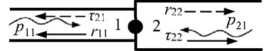
Two connected semi-infinite beams are shown in Fig. 2. In this application, energy flow transmitting coefficients are available through the energy flow transmission coefficient equations. The net flexural energy flow away from a junction of coupled beams with stepped thickness are:

21

{⟨q⟩}_{2}^{+} = τ_{12} {⟨q⟩}_{1}^{+} + r_{22} {⟨q⟩}_{2}^{-},

22

{⟨q⟩}_{1}^{-} = r_{11} {⟨q⟩}_{1}^{+} + τ_{21} {⟨q⟩}_{2}^{-},

where $τ_{i j}$ denotes a flexural energy flow transmitted coefficient in the $j$ th beam owing to the incident flexural wave in the $i$ th beam ( $i$ , $j =$ 1, 2), $r_{i i}$ denotes a flexural energy flow reflected coefficient in the $i$ th beam owing to the incident flexural wave in the $i$ th beam. From reciprocity, $τ_{i j} = τ_{j i}$ and $r_{i i} = r_{j j}$ . On left side of the junction in Fig. 2, node 1 belongs to the finite element 1, and on right side of the junction, node 2 belongs to the finite element 2. At the junction, the net energy flow of nodes 1 and 2 are expressed as the difference between the positive and negative movement energy flow:

23

q_{1} = q_{1}^{+} - q_{1}^{-},

24

q_{2} = q_{2}^{+} - q_{2}^{-},

where:

25

q_{i}^{+} = c_{g i} e_{i}^{+},

26

q_{i}^{-} = c_{g i} e_{i}^{-} .

In Eqs. (25) and (26), the subscript $i$ is the node number ( $i =$ 1, 2), $q_{i}^{+}$ and $q_{i}^{-}$ are the positive and negative movement energy flow in the $i$ th beam respectively, $c_{g i}$ is the group speed of flexural wave in the $i$ th beam.

Substituting Eq. (22) into Eq. (23), a relationship can be obtained as:

27

q_{1} = c_{g 1} (1 - r_{11}) e_{1}^{+} - c_{g 2} τ_{21} e_{2}^{-} .

Since the energy flow values at the junction are continuous, a continuity relationship exists as:

28

q_{1} + q_{2} = 0 .

From Eq. (28), the energy flow at node 2 is the negative of energy flow at node 1. Thus, the energy flow at node 2 is:

29

q_{2} = - c_{g 1} (1 - r_{11}) e_{1}^{+} - c_{g 2} τ_{21} e_{2}^{-} .

In matrix form, Eqs. (27) and (29) can be written as:

30

\{\begin{array}{l} q_{1} \\ q_{2} \end{array}\} = {[P]}_{2 \times 2} \{\begin{array}{l} e_{1}^{+} \\ e_{2}^{-} \end{array}\},

where:

31

{[P]}_{2 \times 2} = [\begin{matrix} c_{g 1} (1 - r_{11}) & - c_{g 2} τ_{21} \\ - c_{g 1} (1 - r_{11}) & c_{g 2} τ_{21} \end{matrix}] .

Next, the energy density values of element nodes at the junction can be written in terms of positive and negative movement energy density. At the junction, the total energy density at nodes 1 and 2 can be expressed as:

32

e_{1} = e_{1}^{+} - e_{1}^{-},

33

e_{2} = e_{2}^{+} - e_{2}^{-} .

Substituting Eqs. (25) and (26), and Eqs. (21) and (22) into Eqs. (32) and (33), the relationships can be obtained as:

34

e_{1} = (1 + r_{11}) e_{1}^{+} + \frac{c_{g 2}}{c_{g 1}} τ_{21} e_{2}^{-},

35

e_{2} = \frac{c_{g 1}}{c_{g 2}} τ_{12} e_{1}^{+} + (1 + r_{22}) e_{2}^{-} .

In matrix form, Eqs. (34) and (35) can be written as:

36

\{\begin{array}{l} e_{1} \\ e_{2} \end{array}\} = {[E]}_{2 \times 2} \{\begin{array}{l} e_{1}^{+} \\ e_{2}^{-} \end{array}\},

where:

37

{[E]}_{2 \times 2} = [\begin{matrix} 1 + r_{11} & \frac{c_{g 2}}{c_{g 1}} τ_{21} \\ \frac{c_{g 1}}{c_{g 2}} τ_{12} & 1 + r_{22} \end{matrix}] .

Now, the relationships given by Eqs. (30) and (37) are combined so that the nodal energy flow at the junction can be represented over the nodal energy density at the junction. In matrix form, nodal values of energy flow are:

38

\{\begin{array}{l} q_{1} \\ q_{2} \end{array}\} = {[J]}_{2 \times 2} \{\begin{array}{l} e_{1} \\ e_{2} \end{array}\},

where:

39

{[J]}_{2 \times 2} = {[P]}_{2 \times 2} {[E]}_{2 \times 2}^{- 1} = \frac{1}{2 (r_{11} + r_{22})} [\begin{matrix} 2 c_{g 1} τ_{12} & - 2 c_{g 2} τ_{21} \\ - 2 c_{g 1} τ_{12} & c_{g 2} τ_{21} \end{matrix}] .

Eq. (39) is the junction element matrix equation for the propagating wave type in two coupled elements. Adding Eq. (39) into Eq. (19), the equilibrium equation in terms of the nodal energy density is:

40

[[\begin{array}{l} K_{1}^{(e)} \\ K_{2}^{(e)} \end{array}] + J] \{\begin{array}{l} e_{1}^{(e)} \\ e_{2}^{(e)} \end{array}\} = \{\begin{array}{l} π_{1}^{(e)} \\ π_{2}^{(e)} \end{array}\} + \{\begin{array}{l} B_{1}^{(e)} \\ B_{2}^{(e)} \end{array}\},

where $K_{1}^{(e)}$ is the stiffness-mass matrix of element 1, and $K_{2}^{(e)}$ is the stiffness-mass matrix of element 2, $J$ is a coupled matrix calculating the energy flow at the junction, $e_{1}^{(e)}$ is the energy density of the element 1, and $e_{2}^{(e)}$ is the energy density of the element 2, $π_{1}^{(e)}$ is the power input to the element 1, and $π_{2}^{(e)}$ is the power input to the element 2, $B_{1}^{(e)}$ is the energy flow at the boundary of element 1, and $B_{2}^{(e)}$ is the energy flow at the boundary of element 2. In this paper, the cross-section areas at the junction of two coupled beams with stepped thickness are not equal. The different cross-section areas make nodal values of energy density discontinuous. The junction equations at the all junctions are assembled into a global equation. A global EFEA equation for coupling beams with stepped thickness and variable cross-section is obtained as:

41

[K + J C] e = π_{i n} + B,

where $J C$ is a global junction matrix containing junction matrices at the all junctions.

Fig. 2Node placement at the junction of coupled structural elements

3. Applications

Firstly, the convergence study is achieved by analyzing the relation between element number and energy density through a uniform beam. Then, the errors between EFEA and analytical results are analyzed. Secondly, EFEA, analytical and FEA approaches are utilized to predict the structural response of a uniform beam with the boundaries of one free and one clamped at each end. These approaches also applied to a non-uniform beam. The EFEA results are compared with analytical and FEA results to verify the equation in terms of energy density in the EFEA approach. Finally, the junction equation is applied to coupled beams with stepped thickness. In all applications, the element sizes are approached to or greater than one sixth of the wavelength. This request is satisfied with the calculation accuracy.

3.1. The convergence study

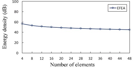
A uniform beam shown in Fig. 1 is utilized to analyze the convergence of the EFEA method. Parameters are employed as below: $L =$ 1 m, $E =$ 2×10¹¹ N/m², $I =$ 3.217×10^-9 m⁴, $ρ =$ 7800 kg/m³, $S =$ 2.011×10^-4 m², $F_{0} =$ 20 N, $η =$ 0.005, $f =$ 50,000 Hz. Fig. 3 presents the nodal values of energy density at the center ( $x = L / 2$ ) of the beam tend to be uniformed and converged as the number of elements increase. Table 1 presents that the error is approximated to 2.78 % when the element number increases to 36 (the size of element length closes to $λ /$ 4, typically $λ$ is the length of flexural wave), and the error closes to zero when the element number increases to 48. The results present the convergence speed of the EFEA method is relatively quick, and this method is also used to calculate the energy density of vibrational structures at high frequency.

Table 1Errors between EFEA and Exact results at x=L/2 (f= 50,000 Hz, η= 0.005)

No.	Element number	EFEA (dB)	Exact (dB)	Error (%)
1	12	51.287	45.042	13.84
2	20	48.940	45.042	8.65
3	28	47.421	45.042	5.28
4	36	46.297	45.042	2.78
5	44	45.404	45.042	0.80
6	48	45.048	45.042	0.00

Fig. 3The EFEA results of the free-clamped uniform beam at x=L/2 when the structural damping is 0.005 and the analysis frequency is 50,000 Hz. The reference energy density is 1×10-12 J/m2

The EFEA results of the free-clamped uniform beam at x=L/2 when the structural damping is 0.005 and the analysis frequency is 50,000 Hz. The reference energy density is 1×10-12 J/m2

3.2. A uniform beam

A uniform beam shown in Fig. 1 is subjected to the transverse excitation $F_{0} e^{j ω t}$ with the amplitude $F_{0} =$ 20 N which is acted on the free end. This uniform beam is employed to predict the structural respone through the EFEA, analytical and FEA approaches. Beam parameters are given as: $L =$ 1 m, $E =$ 2×10¹¹ N/m², $I =$ 3.217×10^-9 m⁴, $ρ =$ 7800 kg/m³, $S =$ 2.011×10^-4 m².

Fig. 4 presents the Exact and EFEA results at $x =$ $L /$ 2 under various excitation frequencies and the structural damping $η =$ 0.05. The presented EFEA results are the frequency average of analytical results which are described by “exact” results in the current investigation. The presented EFEA results are independent of the element resonant states. The analytical results are acquired without space- and time-averaged, and the wavelengths are small at higher frequencies. Therefore, at higher frequencies, the variance of analytical results tends to be uniform and the presented EFEA solutions are analogous to the analytical results.

Fig. 4The EFEA results of the free-clamped uniform beam at x=L/2 for various frequencies and the structural damping η= 0.05. The reference energy density is 1×10-12 J/m2

The EFEA results of the free-clamped uniform beam at x=L/2 for various frequencies and the structural damping η= 0.05. The reference energy density is 1×10-12 J/m2

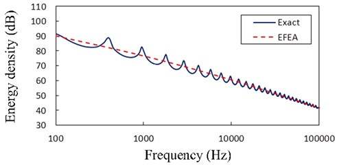
Fig. 5 presents the EFEA results when the frequency is 20,000 Hz and structural damping loss factors are 0.005, 0.01, 0.05, respectively. According Eq. (15), if the structural damping becomes small, the values in the stiff-matrix get big and the values in the mass-matrix get small. The presented EFEA results decrease slowly with distance from the free end and approach to zero near the clamped end. As the structural damping loss factor decreases from 0.05 to 0.005, the value of energy density decreases when the frequency is 20,000 Hz.

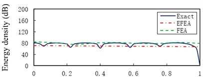
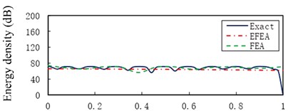
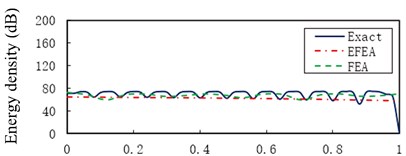
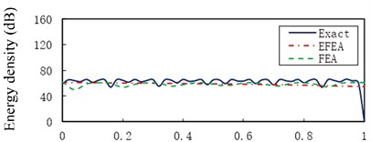
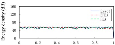
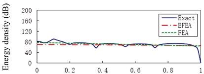
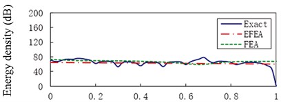
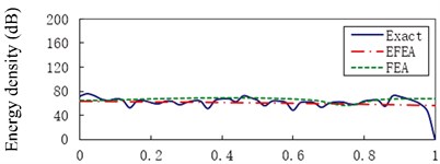
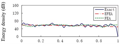
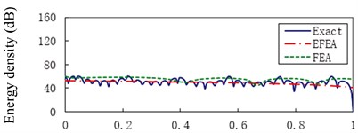
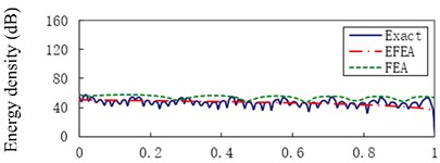
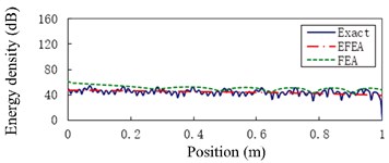
Fig. 6 presents the Exact, EFEA and FEA results of the uniform beam during the structural damping 0.005 and excitation frequencies 1000 Hz through 80,000 Hz, respectively. The energy variables are spatially averaged and time averaged, so presented EFEA results are smoothed. The presented EFEA results are independent of the element resonant states. Even if EFEA results are smoothed, the results also effectively reflect the global variation of analytical results, for the evanescent wave is neglected in the EFEA models. As the excitation frequency increases from 1000 Hz to 80,000 Hz, the averaged energy density decreases from 77.23 dB to 45.18 dB. The EFEA results are compared with analytical and FEA results. In Fig. 6(a), the Exact results are between EFEA and FEA results. At the lower frequency, the FEA approach is qualified to analyze the vibration response of the uniform beam. In Fig. 6(g), the EFEA results are more similar to the analytical results than FEA results. It is showed the EFEA approach is qualified to analyze the vibration response of the uniform beam at higher frequency.

Fig. 5The EFEA results of the free-clamped uniform beam under the analysis frequency f= 20,000 Hz and structural damping loss factors (η= 0.005, 0.01, 0.05). The reference energy density is 1×10-12 J/m2

The EFEA results of the free-clamped uniform beam under the analysis frequency f= 20,000 Hz and structural damping loss factors (η= 0.005, 0.01, 0.05). The reference energy density is 1×10-12 J/m2

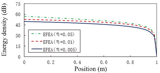
Fig. 6The Exact, EFEA and FEA results of a uniform beam (η= 0.005): a) f= 1000 Hz, b) f= 3000 Hz, c) f= 5000 Hz, d) f= 11,000 Hz, e) f= 30,000 Hz, f) f= 50,000 Hz, g) f= 80,000 Hz. The reference energy density is 1×10-12 J/m2

The Exact, EFEA and FEA results of a uniform beam (η= 0.005): a) f= 1000 Hz, b) f= 3000 Hz, c) f= 5000 Hz, d) f= 11,000 Hz, e) f= 30,000 Hz, f) f= 50,000 Hz, g) f= 80,000 Hz. The reference energy density is 1×10-12 J/m2

a)

b)

c)

d)

e)

3.3. A non-uniform beam

A non-uniform beam drawn in Fig. 7 is taken into account. A harmonic excitation $F_{0} e^{j ω t}$ with the amplitude $F_{0} =$ 20 N is acted on the free end. The non-uniform beam parameters are: $L =$ 1 m, $E =$ 2×10¹¹ N/m², $I_{x 1 = 0} =$ 3.217×10^-9 m⁴, $I_{x 2 = L} =$ 1.628×10^-8 m⁴, $ρ =$ 7800 kg/m³, $S_{x 1 = 0} =$ 2.011×10^-4 m², $S_{x 2 = L} =$ 4.524×10^-4 m², $η =$ 0.005.

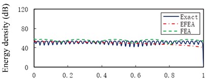
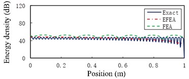
Fig. 8 presents the Exact, EFEA and FEA results of a non-uniform beam under the structural damping 0.005 and analysis frequencies 1000 Hz through 80,000 Hz, respectively. Similar to the uniform beam, the FEA results are effective at lower frequencies. However, the EFEA results in the non-uniform beam are closer to the analytical results than FEA results at higher frequencies. In Fig. 8(e)-(g), EFEA results are smaller than FEA results because more energies are dissipated in the EFEA model due to structural damping. As the excitation frequency increases from 1000 Hz to 80,000 Hz, the averaged energy density decreases from 72.44 dB to 43.92 dB.

Fig. 7A non-uniform beam

3.4. Free-clamped beams with stepped thickness and variable cross-section

In this section and next section, the junction formulation is employed to build the EFEA model at the junction across the beams with steeped thickness and variable cross-section. In order to use the energy flow at the junction to establish the junction expression, the node at the junction should be copied into two nodes.

Fig. 9 presents the free-clamped beams with stepped thickness and variable cross-section, which is loaded by an input excitation $F_{0} e^{j ω t}$ with $F_{0} =$ 1 N. Such a model is employed to predict the analytical, EFEA and FEA results. The properties of coupled beams are: $L_{a}$ = $L_{b}$ = $L_{c}$ = 1/3 m, $E_{a}$ = $E_{b}$ = $E_{c}$ = 2×10¹¹ N/m², $I_{x 1}$ = 1.88×10^-9 m⁴, $I_{x 2 L}$ = 3.22×10^-9 m⁴, $I_{x 2 R}$ = 5.15×10^-9 m⁴, $I_{x 3 L}$ = 7.85×10^-9 m^4, $I_{x 3 R}$ = 1.15×10^-8 m⁴, $I_{x 4}$ = 1.63×10^-8 m⁴, $ρ_{a}$ = $ρ_{a}$ = 7800 kg/m³, $S_{x 1}$ = 1.54×10^-4 m², $S_{x 2 L}$ = 2.01×10^-4 m², $S_{x 2 R}$ = 2.54×10^-4 m², $S_{x 3 L}$ = 3.14×10^-4 m², $S_{x 3 R}$ = 3.80×10^-4 m², $S_{x 4}$ = 4.51×10^-4 m², $η_{a}$ = $η_{b}$ = $η_{c}$ =0.03 or 0.05.

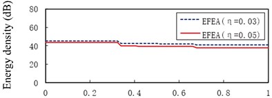
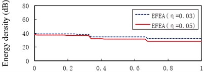
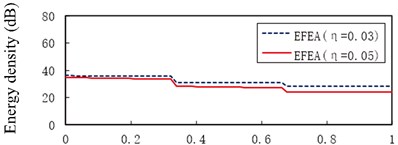
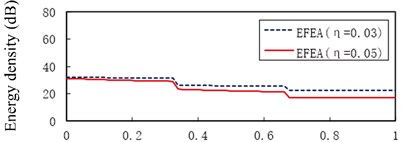
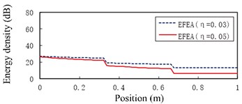
Fig. 10 presents the EFEA results of the free-clamped beams when the frequencies are 3000 Hz, 9000 Hz, 15,000 Hz, 30,000 Hz and 80,000 Hz, respectively. The value of energy density decreases as the any part of beams is away from the free end of beam A. There are two sudden changes at the two junctions, and the jump at $x = L_{a}$ is larger than another jump at $x = L_{a} + L_{b}$ . At the given frequency, the level of energy density at the structural damping 0.03 is higher than that at the structural damping 0.05, shown in Fig. 10(a) through Fig. 10(e). At the given structural damping, the level of energy density at the frequency 3000 Hz is higher than that at the frequency 9000 Hz, shown in Fig. 11(a) or Fig. 11(b). It is showed that the value of energy density decreases as the structural damping or the excitation frequency increases. Table 2 presents the EFEA results at the discontinuities. The difference of energy density at the junction under the structural damping 0.05 is larger than that at the structural damping 0.03 at $x = L_{a}$ . It is shown that more energies are dissipated by the increasing structural damping. Under the structural damping 0.03, the difference of energy density is from 2.86 dB to 5.82 dB when the excittion frequency is from 1000 Hz to 80,000 Hz. Also, the difference is from 3.80 dB to 6.36 dB under the structural damping 0.05. This phenomenon indicates that at the given structural damping the difference of energy density becomes big as the frequency increases. Eq. (38) which is a junction equation is used to deal with the discontinuity problem of energy density at the junction of beams with stepped thickness. The results at the junction of beams with steeped thickness and variable cross-section show the validity of the EFEA approach.

Fig. 8The Exact, EFEA and FEA results of a uniform beam: a) f=1000 Hz, b) f= 3000 Hz, c) f= 5000 Hz, d) f= 11,000 Hz, e) f= 30,000 Hz, f) f= 50,000 Hz, g) f= 80,000 Hz. The reference energy density is 1×10-12 J/m2

The Exact, EFEA and FEA results of a uniform beam: a) f=1000 Hz, b) f= 3000 Hz, c) f= 5000 Hz, d) f= 11,000 Hz, e) f= 30,000 Hz, f) f= 50,000 Hz, g) f= 80,000 Hz. The reference energy density is 1×10-12 J/m2

a)

b)

c)

d)

e)

f)

g)

Table 2The EFEA results at the discontinuities

Case	$x = L_{a L}$ ( $η =$ 0.03)	$x = L_{a R}$ ( $η =$ 0.03)	Difference ( $η =$ 0.03)	$x = L_{a L}$ ( $η =$ 0.05)	$x = L_{a R}$ ( $η =$ 0.05)	Difference ( $η =$ 0.05)
a	45.25	42.39	2.86	43.54	39.74	3.80
b	38.64	34.77	3.87	36.82	31.97	4.85
c	35.53	31.17	4.36	33.60	28.29	5.31
d	31.24	26.23	5.01	29.06	23.22	5.84
e	24.90	19.08	5.82	22.06	15.70	6.36
Note: $L_{a L}$ is the left of length $L_{a}$ , $L_{a R}$ is the right of length $L_{a}$

Fig. 9Free-clamped beams with stepped thickness and variable cross-section

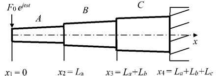
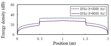
Fig. 10The EFEA results of free-clamped beams at different frequencies: a) f= 3000 Hz, b) f= 9000 Hz, c) f= 15,000 Hz, d) f= 30,000 Hz, e) f= 80,000 Hz. The reference energy density is 1×10-12 J/m2

The EFEA results of free-clamped beams at different frequencies: a) f= 3000 Hz, b) f= 9000 Hz, c) f= 15,000 Hz, d) f= 30,000 Hz, e) f= 80,000 Hz. The reference energy density is 1×10-12 J/m2

a)

b)

c)

d)

e)

Fig. 11The EFEA results of free-clamped beams under different structural damping: a) η= 0.03, b) η= 0.05. The reference energy density is 1×10-12 J/m2

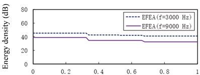
a)

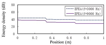
b)

3.5. Two-end-clamped beams with stepped thickness and variable cross-section

Two-end-clamped beams with stepped thickness and variable cross-section are shown in Fig. 12. A harmonic point force $F_{0} e^{j ω t}$ with $F_{0} =$ 1 N is enforced on the center of beam B. The two-end-clamped beams are adopted to acquire the analytical, EFEA and FEA solutions. The properties of coupled beams are: $L_{a} = L_{c}$ = 0.5 m, $L_{b} =$ 1 m, $E_{a} = E_{b}$ = $E_{c} =$ 2×10¹¹ N/m², $I_{x 1} =$ 1.63×10^-8 m⁴, $I_{x 2 L} =$ 7.85×10^-8 m⁴, $I_{x 2 R} = I_{x 3 L} =$ 5.153×10^-9 m⁴, $I_{x 3 R} =$ 7.85×10^-9 m⁴, $I_{x 4} =$ 1.63×10^-8 m⁴, $ρ_{a} = ρ_{b} = ρ_{c} =$ 7800 kg/m³, $η_{a} = η_{b} = η_{c} =$ 0.005 or 0.05, $S_{x 1} =$ 4.52×10^-4 m², $S_{x 2 L} =$ 3.14×10^-4 m², $S_{x 2 R} = S_{x 3 L} =$ 2.54×10^-4 m², $S_{x 3 R} =$ 3.14×10^-4 m², $S_{x 4} =$ 4.52×10^-4 m².

Fig. 12Two-end-clamped beams with stepped thickness and variable cross-section

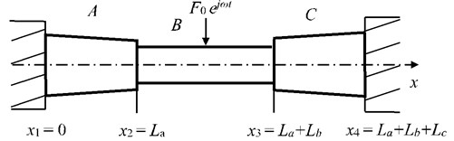
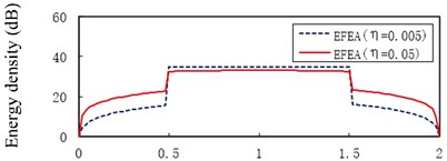
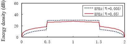
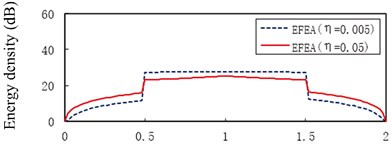
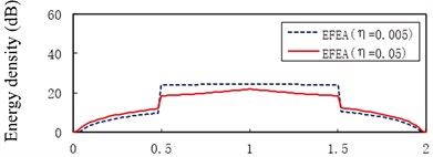
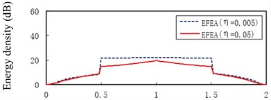
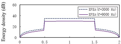
Fig. 13 presents the EFEA results for two-end-clamped beams when the frequencies are 3000 Hz, 9000 Hz, 15,000 Hz, 30,000 Hz, 50,000 Hz and 80,000 Hz respectively. The value of energy density decreases as the any part of beams is away from the harmonic excitation point at beam B. Similar to the free-clamped beams in the section 3.4, two jumps of EFEA results exist in the junctions. When the frequencies are 3000 Hz through 80,000 Hz, the level of energy density of beam B at the hysteresis damping 0.005 is higher than that at the hysteresis damping 0.05.

Fig. 13The EFEA results of two-end-clamped beams at different excitation frequencies: a) f= 3000 Hz, b) f= 9000 Hz, c) f= 15,000 Hz, d) f= 30,000 Hz, e) f= 50,000 Hz, f) f= 80,000 Hz

The EFEA results of two-end-clamped beams at different excitation frequencies: a) f= 3000 Hz, b) f= 9000 Hz, c) f= 15,000 Hz, d) f= 30,000 Hz, e) f= 50,000 Hz, f) f= 80,000 Hz

a)

b)

c)

d)

e)

f)

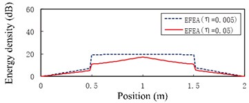
Fig. 14The EFEA results of two-end-clamped beams under different structural damping: a) η= 0.005, b) η= 0.05. The reference energy density is 1×10-12 J/m2

a)

b)

However, the level of energy density of beam A or beam C at hysteresis damping 0.005 is lower than that at the hysteresis damping 0.05 when the frequencies are 3000 Hz through 30,000 Hz, similarly for some part of beam A or beam C at 50,000 Hz in Fig. 13(e). The energy density level of some part of beam A or beam C at the hysteresis damping 0.005 is higher than that at the hysteresis damping 0.05 in Fig. 13(e), similarly for beam A or beam C at 80,000 Hz in Fig. 13(f). This phenomenon results from the boundary conditions and the discontinuities which affect the propagation of flexural wave. Fig. 14 presents the EFEA results when the structural damping is 0.005 and 0.05. When the hysteresis damping is constant, the level of energy density declines as the frequency increases. Table 3 presents the EFEA results at the discontinuities. The change trend of the difference of energy density at the junction is reversely compared with the free-clamped beams in section 3.4. It is caused by the different boundary conditions or geometrical structures. The difference of energy density at the structural damping 0.005 is larger than that at the damping 0.05. For example, in Fig. 13(a) the difference value decreases from 23.22 dB to 9.81 dB at $x = L_{a}$ as the hysteresis damping increases from 0.005 to 0.05. When the structural damping is constant, the difference of energy density decreases as the frequency increases. For example, the difference of energy density at the damping 0.005 is from 23.22 dB under the frequency 3000 Hz to 12.34 dB under 80,000 Hz, similarly from 9.81 dB to 5.84 dB at the damping 0.05. It is showed that the increasing damping or frequency makes the junction dissipate less energies.

Table 3The EFEA results at the discontinuities

Case	$x = L_{a L}$ ( $η =$ 0.005)	$x = L_{a R}$ ( $η =$ 0.005)	Difference ( $η =$ 0.005)	$x = L_{a L}$ ( $η =$ 0.05)	$x = L_{a R}$ ( $η =$ 0.05)	Difference ( $η =$ 0.05)
a	11.53	34.75	23.22	22.77	32.58	9.81
b	12.90	29.78	16.88	18.36	26.33	7.97
c	11.63	27.42	15.79	15.93	23.18	7.25
d	9.83	24.17	14.34	12.09	18.57	6.48
e	8.43	21.72	13.29	8.75	14.84	6.09
f	7.07	19.41	12.34	5.23	11.07	5.84
Note: $L_{a L}$ is the left of length $L_{a}$ , $L_{a R}$ is the right of length $L_{a}$

4. Conclusions

The paper has focused on energy finite element analysis of vibrating beams with stepped thickness and variable cross-section in mid-to-high frequency range. An energy finite element formulation based on the energy variation and the far field assumption has been proposed specifically for predicting the distribution of energy density of uniform beams. The junction equation deduced from the balance equation of energy flow has provided an effective approach to resolve the problem of discontinuous energy density at the junction of coupled beams with stepped thickness.

The feasibility of the developed energy finite element approach has been validated by employing several design examples under the various excitation frequencies and structural damping loss factors. The convergence study of given example presents the error is approximated to 2.78 % when the size of element length is close to $λ$ /4 (typically $λ$ is the length of flexural wave). Comparing the EFEA solutions with the “exact” and FEA results for uniform and non-uniform beams, the present EFEA solutions are smoothed to represent effectively the global variation of the analytical results at high frequency. At lower frequencies, the FEA results seem to be in accord with the analytical results. However, at higher frequencies the EFEA results are analogous to the analytical results.

In the free-clamped beams with stepped thickness and variable cross-section, two jumps of the EFEA results are on the junctions. The value of energy density decreases as the structural damping or the exciation frequency increases. When the excitation frequency is constant, the difference of energy density at the junction under the structural damping 0.05 is larger than that at the structural damping 0.03. At the given structural damping, the difference of energy density becomes big as the frequency increases. It is show that more energies are dissipated due to the increasing structural damping or excitation frequency.

In the two-end-clamped beams with stepped thickness and variable cross-section, there are also two jumps on the junctions. The level of energy density of beam B at the hysteresis damping 0.005 is higher than that at the hysteresis damping 0.05 when the frequencies are 3000 Hz through 80,000 Hz. However, the level of energy density of beam A or beam C at the hysteresis damping 0.005 is lower than that at the hysteresis damping 0.05 when the frequencies are 3000 Hz through 30,000 Hz, similarly for some part of beam A or beam C at the frequency 50,000 Hz. But the difference of energy density at the junctions decreases as the structural damping or excitation frequency increases. This phenomenon results from the boundary conditions. The difference of energy density at the junction become small as the hysteresis damping or frequency increases. It is showed that the increasing damping or frequency makes the junction dissipate less energies. Thus, EFEA method is a preferential selective approach of energy flow specially for evaluating the distribution of energy density of complicatedly vibrating structures at high frequency when classical approaches become too numerically intensive.

References

Nefske D. J., Sung S. H. Power flow finite element analysis of dynamic systems: basic theory and application to beams. Transactions of the ASME, Vol. 111, Issue 1, 1989, p. 94-100.

Search CrossRef
Zhao X., Vlahopoulos N. A basic hybrid finite element formulation for mid-frequency analysis of beams connected at an arbitrary angle. Journal of Sound and Vibration, Vol. 269, Issue 1, 2004, p. 135-164.

Publisher
Hambric S. A., Sung S. H., Nefske D. J. Engineering Vibroacoustic Analysis: Methods and Applications. John Wiley & Sons, USA, 2016.

Publisher
Wohlever N. C., Bernhard R. J. Mechanical energy flow models of rods and beams. Journal of Sound and Vibration, Vol. 153, Issue 1, 1992, p. 1-19.

Publisher
Lyon R. H., Maidanik G. Power flow between linearly coupled oscillators. Journal of Acoustical Society of America, Vol. 34, Issue 5, 1962, p. 623-639.

Publisher
Lyon H. Statistical Energy Analysis of Dynamical Systems. The MIT Press, Cambridge, Massachusetts, 1975.

Search CrossRef
Han J. B., Hong S. Y., Song J. H., Kwon H. W. Vibrational energy flow models for the 1-D high damping system. Journal of Mechanical Science and Technology, Vol. 27, Issue 9, 2013, p. 2659-2671.

Publisher
Bernhard R. J., Huff J. E. Structural-acoustic design at high frequency using the energy finite element method. Journal of Sound and Vibration, Vol. 121, Issue 3, 1999, p. 295-301.

Search CrossRef
Vlahopoulos N., Zhao X. Basic development of a hybrid finite element method for mid-frequency computations of structural vibrations. AIAA Journal, Vol. 37, Issue 1, 1999, p. 1495-1505.

Publisher
Lin Z. L., Chen X. L., Zhang B. Energy finite element analysis of vibrating beams at high frequency. International Conference on Information and Automation, Macau SAR, China, 2017, p. 1033-1038.

Search CrossRef
Navazi H. M., Nokhbatolfoghahai A., Ghobad Y., Haddadpour H. Experimental measurement of energy density in a vibrating plate and comparison with energy finite element analysis. Journal of Sound and Vibration, Vol. 375, Issue 4, 2016, p. 289-307.

Publisher
Nokhbatolfoghahai A., Navazi H. M., Ghobaad Y., Haddadpour H. Experimental measurement of energy density of a vibrating beam. Journal of Vibration and Control, 2016, https://doi.org/10.1177/1077546316629596.

Publisher
Kil H. G., Lee B. C., Lee Y. H., Lee H. H., Hong S. Y., Park Y. H., Seo S. H. Experimental study on the energy flow analysis of vibration of an automobile door. SAE Papers 2005-01-2323, 2005.

Publisher
Vlahopoulos N., Zhao X., Allen T. An approach for evaluating power transfer coefficients for spot-welded joints in an energy finite element formulation. Journal of Sound and Vibration, Vol. 220, Issue 1, 1990, p. 135-154.

Publisher
Cremer L., Heckl M. Structure-Borne Sound. Springer-Verlag, Berlin, 1973.

Publisher
Cook R. D., Malkus D. S., Plesha M. E., Witt R. J. Concepts and Applications of Finite Element Analysis. The University of Wisconsin, Madison, 2007.

Search CrossRef
Yang Y. Research on Energy Finite Element Analysis and Its Application to Composite Laminate Plate. Master Thesis, Ningbo University, China, 2014.

Search CrossRef
Kong X. J., Chen H. L., Zhu D. H., Zhang W. B. Study on the validity region of energy finite element analysis. Journal of Sound and Vibration, Vol. 333, Issue 1, 2014, p. 2601-2616.

Publisher

Cited by

Research status and development trend of energy finite element analysis: a review

Miaoxia Xie | Feilong Yao | Ling Li | Yueming Li

(2023)

Prediction of the Transient Local Energy by Energy Finite Element Analysis

Huaizhi Wang | Kaiping Yu | Rui Zhao

(2023)

Energy Flow Analysis of One-Dimensional Structures with Random Properties

Kun Wang | Yu Fu | Jiafu Liu | Qi Zhang | Giuseppe Ruta

(2020)

About this article

Received

10 January 2018

Accepted

20 May 2018

Published

30 September 2018

SUBJECTS

Mechanical vibrations and applications

DOI

https://doi.org/10.21595/jve.2018.19625

Keywords

junction equation

energy flow

structural damping

vibration

variable section

Acknowledgements

This work was partially supported by the National Hightech R&D Program of China (863 Program) (No. 2015AA016403).

Conflict of interest

The authors declare that there is no conflict of interests regarding the publication of this paper.

This is an open access article distributed under the Creative Commons Attribution License, which permits unrestricted use, distribution, and reproduction in any medium, provided the original work is properly cited.

Next article in issue Next

Research article

2024 03 02

An analytical model for the analysis of vibration and energy flow in a clamped stiffened plate using integral transform technique

Hui Guo, Kai Zhang

Review article

2023 01 05

Research status and development trend of energy finite element analysis: a review

Miaoxia Xie, Feilong Yao, Ling Li, Yueming Li

Review article

2017 08 15

Invited Review: Recent developments in vibration control of building and bridge structures

Khaled Ghaedi, Zainah Ibrahim, Hojjat Adeli, Ahad Javanmardi

Research article

2016 08 15

Vibro-acoustic coupled analysis excited by correlated turbulent boundary layer

Yanbin Li, Qingguo Fei, Shaoqing Wu, Peng Zhang, Dong Jiang

Z. Lin, X. Chen, and B. Zhang, “Application of the energy finite element analysis to vibration of beams with stepped thickness and variable cross-section,” Journal of Vibroengineering, Vol. 20, No. 6, pp. 2237–2252, Sep. 2018, https://doi.org/10.21595/jve.2018.19625

Copy Extrica

Copied to clipboard!

TY  - JOUR
DO  - 10.21595/jve.2018.19625
UR  - https://doi.org/10.21595/jve.2018.19625
TI  - Application of the energy finite element analysis to vibration of beams with stepped thickness and variable cross-section
T2  - Journal of Vibroengineering
AU  - Chen, Xiliang
AU  - Lin, Zhili
AU  - Zhang, Bo
PY  - 2018
DA  - 2018/09/30
PB  - JVE International Ltd.
SP  - 2237-2252
IS  - 6
VL  - 20
SN  - 1392-8716
SN  - 2538-8460
ER  - 

Copy Ris

Copied to clipboard!

@article{Chen_2018,
	doi = {10.21595/jve.2018.19625},
	url = {https://doi.org/10.21595/jve.2018.19625},
	year = 2018,
	month = {sep},
	publisher = {{JVE} International Ltd.},
	volume = {20},
	number = {6},
	pages = {2237--2252},
	author = {Xiliang Chen and Zhili Lin and Bo Zhang},
	title = {Application of the energy finite element analysis to vibration of beams with stepped thickness and variable cross-section},
	journal = {Journal of Vibroengineering}
}

Copy Bibtex

Copied to clipboard!

[1]X. Chen, Z. Lin, and B. Zhang, “Application of the energy finite element analysis to vibration of beams with stepped thickness and variable cross-section,” Journal of Vibroengineering, vol. 20, no. 6, pp. 2237–2252, Sep. 2018, doi: 10.21595/jve.2018.19625.

Copy IEEE

Copied to clipboard!

Chen, Xiliang, Zhili Lin, and Bo Zhang. “Application of the Energy Finite Element Analysis to Vibration of Beams with Stepped Thickness and Variable Cross-Section.” Journal of Vibroengineering 20, no. 6 (September 30, 2018): 2237–52. https://doi.org/10.21595/jve.2018.19625.

Copy Chicago

Copied to clipboard!

Application of the energy finite element analysis to vibration of beams with stepped thickness and variable cross-section

Abstract

1. Introduction

2. Basic theory

2.1. Analytical equation

2.2. Energy finite element equation

2.3. Junction equation

3. Applications

3.1. The convergence study

3.2. A uniform beam

3.3. A non-uniform beam

3.4. Free-clamped beams with stepped thickness and variable cross-section

3.5. Two-end-clamped beams with stepped thickness and variable cross-section

4. Conclusions

References

Cited by

About this article

Related Articles